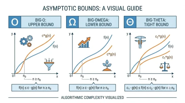
Big-O is the asymptotic upper bound, so it describes the worst case. Big-Omega is the lower bound, so it describes the best case. Big-Theta is a tight bound, meaning the function grows at the same rate from above and below. In short, Big-O caps growth, Big-Omega floors it, and Big-Theta pins it exactly.
Every algorithms course and coding interview eventually circles back to asymptotic notation. Students often memorise Big-O and stop there, then freeze when an examiner asks about the lower bound. The trio of big o vs big omega vs big theta exists because one symbol cannot describe every case of an algorithm.
These three symbols measure how a running time or space cost grows as the input size n gets large. They ignore constants and small inputs on purpose. That abstraction is exactly why they travel so well across machines and languages.
This guide gives you the formal definitions, the plain-English meaning, and a worked example that exposes a common trap. By the end, you will know precisely which notation to reach for and why.
What is asymptotic notation?
Asymptotic notation describes how a function behaves as its input grows toward infinity. In algorithm analysis, that function is usually a running time T(n) or a space cost. We compare T(n) against a simpler reference function g(n), such as n or n squared.
The notation deliberately drops constant factors and lower-order terms. So 3n + 7 and 100n both reduce to the same linear class. This lets us compare algorithms by their growth rate rather than by hardware speed.
Big-O, Big-Omega, and Big-Theta answer three different questions about that growth. Big-O asks how bad it can get, Big-Omega asks how good it can get, and Big-Theta asks whether both answers match. Keeping those questions separate prevents most confusion.
Big-O: the upper bound
Big-O gives an asymptotic upper bound. It promises the function will not grow faster than g(n) once n is large enough. Engineers reach for it most often because it captures the worst case.
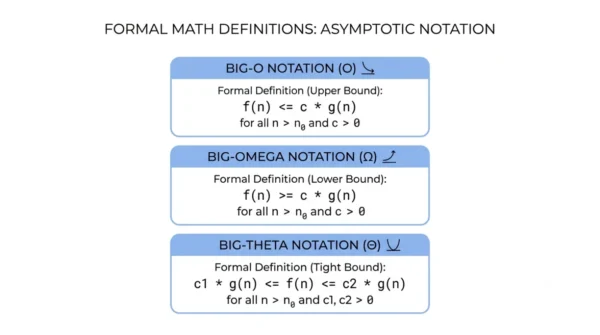
Formally, f(n) = O(g(n)) if and only if there exist positive constants c and n0 such that 0 ≤ f(n) ≤ c · g(n) for all n ≥ n0. In plain English, beyond some starting point n0, the function stays under a scaled copy of g(n).
For example, an algorithm that runs in 3n + 5 steps is O(n). Pick c = 4 and n0 = 5, and the inequality holds for every larger n. The constant and the small offset simply vanish.
Big-Omega: the lower bound
Big-Omega gives an asymptotic lower bound. It promises the function grows at least as fast as g(n) for large n. This describes the best case, the floor that an algorithm cannot beat.
Formally, f(n) = Ω(g(n)) if and only if there exist positive constants c and n0 such that 0 ≤ c · g(n) ≤ f(n) for all n ≥ n0. In words, beyond n0 the function stays above a scaled copy of g(n).
Lower bounds matter when you want to prove a task cannot be done faster. Comparison sorting, for instance, has a proven Ω(n log n) lower bound. No clever comparison sort can ever drop below that floor.
Big-Theta: the tight bound
Big-Theta gives a tight bound. It applies only when the upper and lower bounds match the same growth rate. So f(n) = Θ(g(n)) means the function is both O(g(n)) and Ω(g(n)).
Formally, f(n) = Θ(g(n)) if and only if there exist positive constants c1, c2, and n0 such that 0 ≤ c1 · g(n) ≤ f(n) ≤ c2 · g(n) for all n ≥ n0. The function gets sandwiched between two scaled copies of g(n).
Theta is the most precise notation, yet you can only use it when both bounds agree. The function 3n + 5 is Θ(n) because it is squeezed between, say, 3n and 4n for large n. When best case and worst case differ, no single Theta exists.
Key differences at a glance
| Aspect | Big-O | Big-Omega | Big-Theta |
|---|---|---|---|
| Symbol | O | Ω | Θ |
| Type of bound | Upper bound | Lower bound | Tight bound |
| Case it describes | Worst case ceiling | Best case floor | Exact growth rate |
| Core inequality | f(n) ≤ c · g(n) | f(n) ≥ c · g(n) | c1 · g(n) ≤ f(n) ≤ c2 · g(n) |
| Constants needed | c, n0 | c, n0 | c1, c2, n0 |
| Plain meaning | Grows no faster than g(n) | Grows at least as fast as g(n) | Grows exactly like g(n) |
| How tight | Can be loose or tight | Can be loose or tight | Always tight by definition |
| Implies the others? | No, only the upper side | No, only the lower side | Yes, implies both O and Ω |
| Most common use | Reporting worst-case cost | Proving a problem’s hardness | Stating exact complexity |
| Everyday phrasing | “At most” | “At least” | “Exactly on the order of” |
A worked example without the trap
Linear search is the classic example, but it hides a trap. Searching an unsorted array of n elements runs in Ω(1) in the best case, when the target sits first. It runs in O(n) in the worst case, when the target sits last or is absent.
Because the best case and worst case differ, linear search has no single Big-Theta over all inputs. Calling it Θ(n) is only correct for the worst case specifically, not for the algorithm as a whole. This subtlety trips up many students, so name the case before you name the bound.
For a clean Theta, use an algorithm whose cost does not depend on the input arrangement. Summing every element of an array always touches all n items. So it is O(n), Ω(n), and therefore Θ(n) on every input.
// Summing an array: always touches every element
int total = 0;
for (int i = 0; i < n; i++) {
    total += arr[i];   // runs exactly n times
}
// Best case = worst case = n, so this is Theta(n)
Notice that the loop body runs exactly n times no matter what the array holds. There is no early exit and no skipped work. That uniformity is what lets Big-O, Big-Omega, and Big-Theta collapse onto the same class.
Common complexity classes
Most algorithms fall into a handful of growth classes. The table below lists them from fastest to slowest, with an example operation for each. We have a fuller, applied walkthrough in our dedicated guide on data structure efficiency and time complexity, so this is the quick reference.
| Notation | Name | Typical example |
|---|---|---|
| O(1) | Constant | Array index lookup or a hash map access |
| O(log n) | Logarithmic | Binary search in a sorted array |
| O(n) | Linear | Scanning every element once |
| O(n log n) | Linearithmic | Merge sort or heap sort |
| O(n^2) | Quadratic | A naive nested-loop pair check |
| O(2^n) | Exponential | Brute-force subset enumeration |
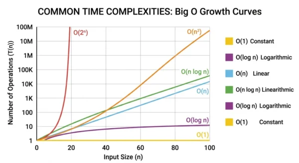
The gap between these classes widens fast as n grows. At a million items, an O(n) scan finishes while an O(n^2) routine grinds for ages. Exponential time becomes hopeless past a few dozen inputs.
When to use which notation
Reach for Big-O when you report a guarantee, since most teams care about the worst case. It answers the practical question of how slow things can get under load. That is why job postings and textbooks lead with it.
Reach for Big-Omega when you argue a problem has a hard floor. It proves that no algorithm can beat a certain speed, which guides where to stop optimising. Lower bounds shine in theory and in algorithm research.
Reach for Big-Theta when best case and worst case match, because it states the exact growth. Use it for tightly characterised routines like merge sort, which is Θ(n log n) on every input. When the cases diverge, describe each case separately instead of forcing one Theta.
Frequently asked questions
Wrapping Up
Asymptotic notation becomes simple once you separate the three questions it answers. Big-O caps growth from above, Big-Omega floors it from below, and Big-Theta pins it exactly when both agree. Always name the case you mean before you name the bound.
Keep the linear-search trap in mind, because it separates students who memorise from those who understand. When best case and worst case differ, report each case rather than forcing one Theta. That habit alone will sharpen your answers in any algorithms exam or interview.
Related reading on DiffStudy:
- Data structure efficiency: understanding time complexity
- Navigating priority queue time complexity
- DFS vs BFS: understanding key differences
- Prim’s vs Kruskal’s algorithm: key differences
- Linear vs non-linear data structures
- Binary tree vs binary search tree
- Explore more CS fundamentals