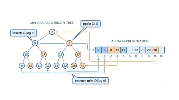
With the usual binary heap, a priority queue does insert in O(log n), peek (find-min) in O(1), and extract-min in O(log n). Building a heap from n items is O(n). The numbers change with the implementation: an unsorted array makes insert O(1) but extract O(n), while a sorted array does the reverse. In short, the binary heap gives the best all-round balance.
Unlike a normal queue, a priority queue serves elements by priority rather than by arrival order. Its time complexity is a staple of DSA courses and interviews, so students need the exact cost of each operation, not vague talk of “efficiency”.
Crucially, those costs depend on how the queue is built. So this guide gives the complexity of every operation, compares the main implementations in a table, explains why the binary heap is O(log n), and lists where priority queues are used.
If Big-O notation is still fuzzy, it helps to review Big-O, Big-Θ, and Big-Ω first.
What is a Priority Queue?
In essence, a priority queue is an abstract data type where every element carries a priority. Instead of first-in-first-out order, the element with the highest priority leaves first. A min-priority queue serves the smallest key first, while a max-priority queue serves the largest.
It supports a few core operations: insert (add an element), peek (read the highest-priority element), and extract (remove and return it). Some versions also support decrease-key, which raises an element’s priority. So the cost of these operations is exactly what “priority queue time complexity” measures.
Time Complexity by Operation
Specifically, with the standard binary heap implementation, the costs are as follows.
- Insert (push): O(log n), because the new element bubbles up the tree.
- Peek (find-min or find-max): O(1), since the top element sits at the root.
- Extract (delete-min or delete-max): O(log n), because the replacement bubbles down.
- Decrease-key: O(log n), as the element bubbles up to its new place.
- Build heap (heapify n items): O(n), which is faster than n separate inserts.
- Search (arbitrary element): O(n), since a heap is not fully ordered.
So the operations you actually queue with, insert and extract, are both O(log n), and reading the front is O(1). That balance is why the heap is the default choice.
Implementation Comparison
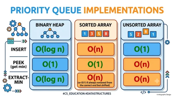
However, the same priority queue has very different costs depending on the underlying structure. The table below shows the worst-case time for each.
| Implementation | Insert | Peek (find-min) | Extract-min | Decrease-key |
|---|---|---|---|---|
| Binary heap | O(log n) | O(1) | O(log n) | O(log n) |
| Binary heap (build) | O(n) for n items | O(1) | O(log n) | O(log n) |
| Unsorted array / list | O(1) | O(n) | O(n) | O(1) |
| Sorted array / list | O(n) | O(1) | O(1) | O(n) |
| Balanced BST | O(log n) | O(log n) | O(log n) | O(log n) |
| Fibonacci heap | O(1)* | O(1) | O(log n)* | O(1)* |
* Fibonacci-heap costs are amortised. Its O(1) insert and decrease-key are what speed up Dijkstra’s and Prim’s algorithms in theory, though the binary heap usually wins in practice on real inputs.
Why the Binary Heap is O(log n)
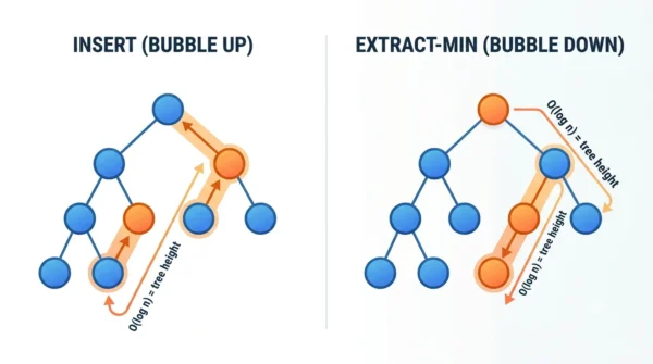
A binary heap is a complete binary tree, so its height is always about log n. That height is the key to the cost.
On insert, you add the element at the bottom, then swap it upward while it beats its parent. Because the path to the root is at most the tree’s height, insert costs O(log n). On extract-min, you remove the root, move the last element to the top, then sink it down to restore order. Again the path is at most log n, so extract is O(log n). Meanwhile, peek just reads the root, which is O(1).
Applications of Priority Queues
Indeed, priority queues power many well-known algorithms and systems, which is why their complexity matters.
- Dijkstra’s shortest path: repeatedly extracts the nearest unvisited node and decreases neighbour keys.
- Prim’s minimum spanning tree: picks the cheapest edge to grow the tree.
- Huffman coding: repeatedly extracts the two lowest-frequency nodes to build the tree.
- Task and CPU scheduling: operating systems run the highest-priority job first.
- A* and other search: expands the most promising node by cost.
- Event-driven simulation: processes the next event by timestamp.
So when speed matters in these algorithms, the O(log n) heap operations are exactly what keep them efficient.
Frequently Asked Questions
Wrapping Up
Priority queue time complexity comes down to the implementation. With a binary heap, insert and extract are O(log n) and peek is O(1), which gives the best balance for most work.
So remember the headline numbers: O(log n) to insert or extract, O(1) to peek, and O(n) to build. With those in hand, you can reason about Dijkstra’s, Prim’s, Huffman coding, and any other algorithm that leans on a priority queue.
Related reading on DiffStudy:


Hi to every one, the contents existing at this web site are actually amazing for people knowledge, well, keep up the nice work fellows.
Hi there! Thanks a lot for your encouraging words! We’re glad you find the content helpful. We’ll definitely keep up the good work.