Cohen-Sutherland vs Liang-Barsky comes down to how each one decides what to keep. Initially, Cohen-Sutherland tags every endpoint with a 4-bit region code. It then runs a bitwise check for a fast accept or reject. When a line genuinely needs clipping, it walks the boundary one edge at a time. So the loop can run more than once. Liang-Barsky instead treats the line as a parametric equation. It solves four inequalities in a single pass, with no looping at all. Because it never repeats work per edge, it usually needs fewer divisions on a line that crosses several boundaries. Even so, Cohen-Sutherland wins when most lines sit entirely inside or entirely outside the window. Those trivial tests are just bitwise operations. In short, for the same input line, both algorithms return exactly the same clipped segment.
Every scene on screen has a boundary. A clip window marks the visible area. Any line reaching past its edges must be trimmed before it gets drawn. So an algorithm has to decide, for every single line, what survives and what gets cut. Cohen-Sutherland and Liang-Barsky are the two classic answers GATE and university courses teach for this problem.
Examiners like this pairing because it rewards precision. They often ask for the outcode bits or the four p and q values. Sometimes they ask for a worked line, clipped by hand against a given window. This guide covers both algorithms in full. It then runs one line through each method, step by step, so you can check your own working against it.
In fact, clipping is not the whole graphics pipeline, just one stage inside it. It follows windowing, which our guide to windowing and clipping in computer graphics covers in full. Once a line survives clipping, it still needs pixels; see DDA vs Bresenham line drawing algorithm for that next stage.
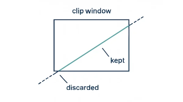
What Line Clipping Has To Decide
A clip window is a rectangle, fixed by four values: xmin, ymin, xmax, and ymax. Anything drawn on screen must stay inside it, or get trimmed until it does.
So, for every line, a clipping algorithm faces exactly three outcomes. Trivial accept happens when both endpoints sit inside the window, so the whole line survives untouched. Trivial reject happens when the line sits entirely past one edge, so nothing survives at all. Partial clip happens when the line crosses one or more edges, so only the inside portion survives.
Telling these three cases apart quickly matters. After all, most scenes contain far more lines than a screen can afford to test in full. Clipping is one of several classic 2D algorithms taught alongside it. Filling a clipped shape is a related problem, covered in flood fill vs boundary fill algorithm.
Cohen-Sutherland and Liang-Barsky both solve this three-way decision. They just reach it through very different arithmetic, as the sections below show.
The Cohen-Sutherland Algorithm
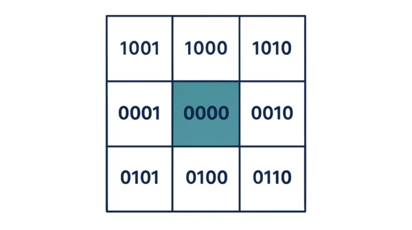
Cohen-Sutherland splits the plane into nine regions. The clip window itself is the centre region, and eight more regions surround it. Every endpoint gets a 4-bit region code, called an outcode, based on where it falls.
The bit order matters, and GATE papers do test it directly:
- Bit 4, value 8, means above the window, the top edge.
- Bit 3, value 4, means below the window, the bottom edge.
- Bit 2, value 2, means right of the window.
- Bit 1, value 1, means left of the window.
A point inside the window gets code 0000, since none of the four bits are set.
Two quick tests handle most lines without any real clipping work:
- Trivial accept: both endpoint codes are 0000. Draw the whole line as it stands.
- Trivial reject: the bitwise AND of the two codes is nonzero. Both endpoints sit outside the same edge, so discard the line entirely.
When neither test fires, the algorithm clips iteratively. Then pick an endpoint whose code is nonzero. Clip it against one window edge that its code flags. Replace that endpoint with the intersection point, then recompute its code. Repeat this loop until a trivial accept or a trivial reject finally fires. A line crossing several edges can send this loop around more than once. The worked example further down shows exactly that.
The intersection formulas depend on which edge is being clipped. Against y = ymax or y = ymin: x = x1 + (x2 − x1)(y_edge − y1)/(y2 − y1). Against x = xmax or x = xmin: y = y1 + (y2 − y1)(x_edge − x1)/(x2 − x1).
Here is the pseudocode.
while True:
    code1 = outcode(x1, y1)
    code2 = outcode(x2, y2)
    if code1 == 0 and code2 == 0:
        accept()
        break
    elif code1 & code2 != 0:
        reject()
        break
    else:
        code_out = code1 if code1 != 0 else code2
        if code_out & TOP:
            x = x1 + (x2 - x1) * (ymax - y1) / (y2 - y1)
            y = ymax
        elif code_out & BOTTOM:
            x = x1 + (x2 - x1) * (ymin - y1) / (y2 - y1)
            y = ymin
        elif code_out & RIGHT:
            y = y1 + (y2 - y1) * (xmax - x1) / (x2 - x1)
            x = xmax
        elif code_out & LEFT:
            y = y1 + (y2 - y1) * (xmin - x1) / (x2 - x1)
            x = xmin
        if code_out == code1:
            x1, y1 = x, y
        else:
            x2, y2 = x, y
Advantages of Cohen-Sutherland.
- Trivial accept and trivial reject are extremely cheap, just a comparison and a bitwise AND.
- It shines whenever most lines are entirely inside or entirely outside the window.
- The outcode idea is easy to visualise, since it maps directly onto the nine regions.
Disadvantages of Cohen-Sutherland.
- It computes intersections one edge at a time, and the loop may repeat.
- A line crossing several edges costs several divisions, one per iteration.
- Every iteration also needs a fresh pair of outcodes, so the bookkeeping adds up.
The Liang-Barsky Algorithm
Liang-Barsky treats a line differently from the start. It writes the line in parametric form: P(t) = P1 + t·ΔP. Here, Δx = x2 − x1 and Δy = y2 − y1, while t runs from 0 to 1.
Clipping the line against all four window edges becomes four inequalities, each shaped like t·pk ≤ qk.
- p1 = −Δx, q1 = x1 − xmin.
- p2 = Δx, q2 = xmax − x1.
- p3 = −Δy, q3 = y1 − ymin.
- p4 = Δy, q4 = ymax − y1.
Each pk and qk pair gets read in one of three ways. If pk = 0, the line runs parallel to that boundary. When that happens and qk is negative, reject the line outright, since it lies entirely on the wrong side. Otherwise, that boundary simply has nothing to say about this line, so skip it.
If pk is negative, the line is entering through that boundary, so t1 = max(t1, qk/pk). If pk is positive, the line is leaving through that boundary, so t2 = min(t2, qk/pk). Start with t1 = 0 and t2 = 1. If t1 ends up greater than t2, reject the line. Otherwise, the clipped endpoints are P(t1) and P(t2).
Here is the pseudocode.
dx = x2 - x1
dy = y2 - y1
p = [-dx, dx, -dy, dy]
q = [x1 - xmin, xmax - x1, y1 - ymin, ymax - y1]
t1, t2 = 0, 1
for k in range(4):
    if p[k] == 0:
        if q[k] < 0:
            reject()
    else:
        t = q[k] / p[k]
        if p[k] < 0: t1 = max(t1, t) else: t2 = min(t2, t) if t1 > t2:
    reject()
else:
    new_x1, new_y1 = x1 + t1 * dx, y1 + t1 * dy
    new_x2, new_y2 = x1 + t2 * dx, y1 + t2 * dy
    accept(new_x1, new_y1, new_x2, new_y2)
Advantages of Liang-Barsky.
- One pass, at most four ratios, and no iteration or loop.
- Parallel lines get handled cleanly, since a zero pk is checked directly.
- It generalises well. Cyrus-Beck applies the very same t1/t2 idea to convex polygons, and Liang-Barsky is the rectangle-window specialisation of it.
Disadvantages of Liang-Barsky.
- Even a line that would trivially accept still needs all four ratios computed.
- The parametric setup takes longer to grasp at first than outcodes do.
- It is built for rectangular windows; a convex polygon window needs Cyrus-Beck instead.
Cohen-Sutherland vs Liang-Barsky: Comparison Table
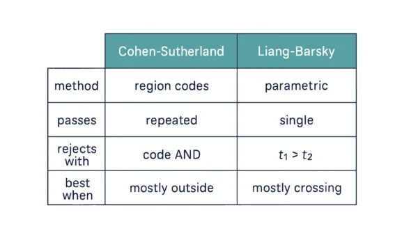
| Aspect | Cohen-Sutherland | Liang-Barsky |
|---|---|---|
| Underlying approach | Region-based outcodes | Parametric line equation |
| Line representation | Raw endpoint coordinates | P(t) = P1 + t·ΔP |
| Trivial accept test | Both outcodes equal 0000 | No separate shortcut; t1 and t2 still get computed |
| Trivial reject test | Bitwise AND of both outcodes is nonzero | t1 > t2 after all four inequalities |
| Number of passes | Iterative; one pass per edge clipped | Single pass, always |
| What gets computed per pass | One outcode pair, one intersection | All four p and q values, once |
| Divisions required | One per clipping iteration | Up to four, never more, in one pass |
| Lines parallel to a boundary | Handled naturally through outcode bits | Explicit case: pk = 0, checked against qk |
| Line crossing several edges | Loop runs several times, once per edge | Still just one pass of four ratios |
| Faster when | Most lines are trivially accepted or rejected | Many lines need genuine partial clipping |
| Ease of implementation | Intuitive once the nine regions click | Needs comfort with parametric equations first |
| Extension to 3D | Extends with extra bits for near/far planes | Extends with two more p/q pairs for z |
| Relationship to Cyrus-Beck | Not related; a separate outcode method | The rectangle-window special case of Cyrus-Beck |
| Typical use | Scenes with mostly inside or outside lines | Scenes with many lines crossing the window |
Worked Example: The Same Line, Both Ways
Take the clip window xmin = 10, ymin = 10, xmax = 80, ymax = 80. The line runs from (5, 5) to (100, 60). Watch the same line pass through both algorithms below.
Cohen-Sutherland needs three states of its loop to finish.
| Step | P1 | Code | P2 | Code |
|---|---|---|---|---|
| 0 | (5, 5) | 0101 | (100, 60) | 0010 |
| 1 | (13.636, 10) | 0000 | (100, 60) | 0010 |
| 2 | (13.636, 10) | 0000 | (80, 48.421) | 0000 |
At step 0, neither code is 0000 and their AND is also 0000, so no trivial decision applies yet. P1’s code flags below and left, so it gets clipped against y = ymin = 10 first, giving x = 13.636. At step 1, P2’s code flags right, so it gets clipped against x = xmax = 80, giving y = 48.421. At step 2, both codes read 0000, so the algorithm accepts.
Liang-Barsky works the same line with Δx = 95 and Δy = 55.
| k | pk | qk | qk/pk | Action |
|---|---|---|---|---|
| 1 | −95 | −5 | 0.0526 | Entering, t1 = 0.0526 |
| 2 | 95 | 75 | 0.7895 | Leaving, t2 = 0.7895 |
| 3 | −55 | −5 | 0.0909 | Entering, t1 = 0.0909 |
| 4 | 55 | 75 | 1.3636 | Leaving, t2 stays 0.7895 |
After all four rows, t1 = 0.0909 and t2 = 0.7895. Since t1 is not greater than t2, the line is accepted. At t1, x = 5 + 0.0909(95) = 13.636 and y = 5 + 0.0909(55) = 10. At t2, x = 5 + 0.7895(95) = 80 and y = 5 + 0.7895(55) = 48.42.
Look closely at both results. Cohen-Sutherland and Liang-Barsky return exactly the same clipped segment, (13.636, 10) to (80, 48.421). However, they reached it through very different work. Cohen-Sutherland needed two clipping iterations. Liang-Barsky needed just one pass of four ratios. That single contrast is the whole argument between them, and the next section builds on it.
Why Liang-Barsky Usually Does Less Work
In the worked example above, Cohen-Sutherland actually needed fewer divisions. It took two, against Liang-Barsky’s four. That is not a mistake, and it is not the usual case either. It happened only because this particular line crossed just two window edges.
Push the same line through a window where it crosses three or four edges instead, and the picture changes. Cohen-Sutherland keeps iterating, since every extra edge means another loop, another division, and another pair of recomputed outcodes. Liang-Barsky never exceeds four ratio computations, no matter how many edges the line actually crosses. All four boundaries get checked in that same single pass.
So the fair comparison is not divisions alone, but divisions relative to how much clipping a line actually needs. When a scene is full of lines that need real, multi-edge clipping, Liang-Barsky’s flat four-ratio cost usually wins. When a scene is full of lines that are already fully inside or fully outside the window, Cohen-Sutherland wins instead. Its trivial tests cost nothing more than a bitwise AND.
Overall, neither algorithm is faster in every case. The right choice depends on what the lines in a given scene actually look like.
Code Example
Below is a working Python version of both algorithms, clipping the same line from the worked example above. Run it, and check the printed endpoints against the tables further up.
def cohen_sutherland_clip(x1, y1, x2, y2, xmin, ymin, xmax, ymax):
    LEFT, RIGHT, BOTTOM, TOP = 1, 2, 4, 8

    def out_code(x, y):
        code = 0
        if x < xmin: code |= LEFT elif x > xmax:
            code |= RIGHT
        if y < ymin: code |= BOTTOM elif y > ymax:
            code |= TOP
        return code

    while True:
        code1 = out_code(x1, y1)
        code2 = out_code(x2, y2)
        if code1 == 0 and code2 == 0:
            return (round(x1, 3), round(y1, 3), round(x2, 3), round(y2, 3))
        if code1 & code2 != 0:
            return None
        code_out = code1 if code1 != 0 else code2
        dx = x2 - x1
        dy = y2 - y1
        if code_out & TOP:
            x = x1 + dx * (ymax - y1) / dy
            y = ymax
        elif code_out & BOTTOM:
            x = x1 + dx * (ymin - y1) / dy
            y = ymin
        elif code_out & RIGHT:
            y = y1 + dy * (xmax - x1) / dx
            x = xmax
        else:
            y = y1 + dy * (xmin - x1) / dx
            x = xmin
        if code_out == code1:
            x1, y1 = x, y
        else:
            x2, y2 = x, y


def liang_barsky_clip(x1, y1, x2, y2, xmin, ymin, xmax, ymax):
    dx = x2 - x1
    dy = y2 - y1
    p = [-dx, dx, -dy, dy]
    q = [x1 - xmin, xmax - x1, y1 - ymin, ymax - y1]
    t1, t2 = 0.0, 1.0
    for pk, qk in zip(p, q):
        if pk == 0:
            if qk < 0:
                return None
            continue
        t = qk / pk
        if pk < 0: t1 = max(t1, t) else: t2 = min(t2, t) if t1 > t2:
        return None
    nx1, ny1 = x1 + t1 * dx, y1 + t1 * dy
    nx2, ny2 = x1 + t2 * dx, y1 + t2 * dy
    return (round(nx1, 3), round(ny1, 3), round(nx2, 3), round(ny2, 3))


print("Cohen-Sutherland:", cohen_sutherland_clip(5, 5, 100, 60, 10, 10, 80, 80))
print("Liang-Barsky:", liang_barsky_clip(5, 5, 100, 60, 10, 10, 80, 80))

# Cohen-Sutherland: (13.636, 10, 80, 48.421)
# Liang-Barsky: (13.636, 10.0, 80.0, 48.421)
Notice what each function actually loops over. cohen_sutherland_clip keeps looping while a code stays nonzero, recomputing outcodes each time. Meanwhile, liang_barsky_clip walks its four p and q pairs exactly once and never loops back. In short, that structural difference is the whole lesson in source-code form.
When to Use Which
Use Cohen-Sutherland when most lines sit entirely inside or outside the clip window. Indeed, its bitwise trivial tests cost almost nothing. Paying for a full clip only on the rare line that truly needs it is a good trade.
Use Liang-Barsky when many lines genuinely need partial clipping. Its flat four-ratio cost never grows with the number of edges crossed. It also suits situations already working in parametric form. Once a line clears clipping, it still needs mapping onto the device viewport. See viewport vs window in computer graphics for that mapping. Clipping itself usually sits downstream of the earlier coordinate pipeline; for that bigger picture, see geometric transformation vs coordinate transformation.
Interview Questions
Frequently Asked Questions
Wrapping Up
Cohen-Sutherland and Liang-Barsky both decide what survives a clip window. For the same input line, they agree on the answer. Cohen-Sutherland reaches it with region outcodes and a loop that may run more than once. Liang-Barsky reaches it with a parametric line and exactly one pass of four ratios.
Remember the essentials for your exam. Trivial reject in Cohen-Sutherland uses AND, never OR. Liang-Barsky is the rectangle-window case of the broader Cyrus-Beck idea. Neither algorithm wins every time; the right pick depends on whether a scene’s lines are mostly trivial or mostly partial.
Related reading on DiffStudy:
- Windowing vs Clipping in Computer Graphics
- DDA vs Bresenham Line Drawing Algorithm
- Viewport vs Window in Computer Graphics
- Geometric Transformation vs Coordinate Transformation
- CS Fundamentals hub