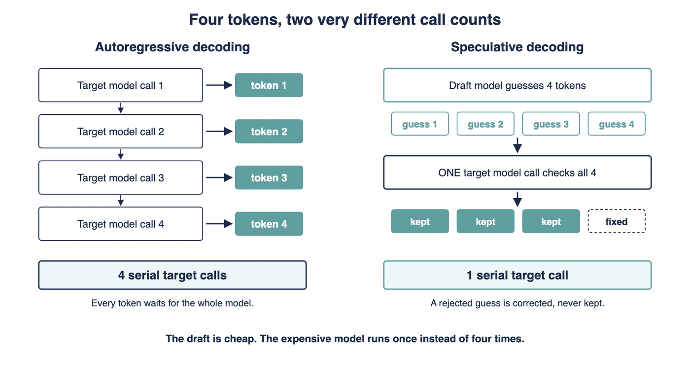
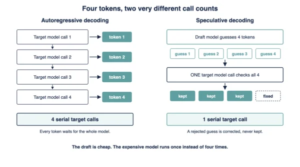
Autoregressive decoding calls the large model once per output token, serially. Speculative decoding drafts several tokens with a small model. It then checks every draft in one parallel pass of the large model. Leviathan and colleagues (Google, 2022) prove the output distribution is unchanged. Chen and colleagues (DeepMind, 2023) call the same idea speculative sampling, measured against autoregressive sampling on a 70B Chinchilla model. Both papers report speedups near “2X-3X”, using more total arithmetic to save serial steps, not less.
A large language model predicts one token, reads that token back in, then predicts the next one. That loop repeats for every token in a reply. Autoregressive decoding is exactly this loop, run start to finish.
Speculative decoding breaks the loop without changing what it computes. A small model drafts ahead of the large one. The large model then checks the draft in a single pass, rather than one token at a time.
This guide reads two papers directly: Leviathan and colleagues from Google, and Chen and colleagues from DeepMind. Both introduce the same trick under different names, and that naming gap trips up plenty of readers.
Why Decoding Is the Slow Part
Training a large model is slow too, though decoding has its own separate problem. Every reply forces the model through its loop again, one token per pass.
That loop is serial by construction. Step two cannot start until step one produces an actual token. The model needs that exact token as its next input. A reply of length L therefore takes L separate passes, run one after another, never in parallel.
Arithmetic is not actually the constraint here, and both papers say so directly. Leviathan and colleagues write that “inference from large models is often not bottlenecked on arithmetic operations, but rather on memory bandwidth and communication, so additional computation resources might be available”. Chen and colleagues, at DeepMind, put it more bluntly: “Transformer sampling is typically memory bandwidth bound”.
So the chips sit partly idle during ordinary decoding. Spare compute exists, yet a serial loop cannot use it. That mismatch is the opening speculative decoding walks through.
How Autoregressive Decoding Works
Autoregressive decoding is the default recipe behind almost every deployed large language model. Predict a token. Feed it back into the model. Predict the next one.
Decoder-only stacks run this loop by design, the same family our BERT vs GPT guide contrasts against encoder stacks. GPT-style models generate exactly one token per forward pass, with no shortcut around it.
Each pass depends completely on the one before it. Nothing later can start early, since the model has not yet produced the token it needs as input. Our diffusion LLM vs autoregressive guide covers this same pattern. It looks at models that avoid the loop, from an entirely different angle.
Chen and colleagues name this baseline autoregressive sampling, or ArS, in their own notation. It becomes the “1x” row in every comparison table. Every other row gets measured against it.
How Speculative Decoding Works
Speculative decoding keeps the one-token-at-a-time guarantee while breaking the one-token-at-a-time pace. A small model runs ahead. A large model checks its work in one pass.
Leviathan and colleagues call the small model the approximation model, written Mq. They call the large model the target model, written Mp. Chen and colleagues, working independently at DeepMind, call the small one the draft model instead. Their whole method is speculative sampling, or SpS, set directly against autoregressive sampling, or ArS. Same two roles, different labels, and readers moving between the papers meet both sets of terms.
The loop has three moves each round. First, the small model proposes several tokens in a row, cheaply and on its own. Second, the large model scores every proposed token in one parallel pass, rather than one token at a time. Third, a rejection rule decides which proposed tokens actually survive.
Chen states the reason this works in one line: “the latency of parallel scoring of short continuations, generated by a faster but less powerful draft model, is comparable to that of sampling a single token from the larger target model”. Scoring several candidates costs about what scoring one token already costs.
When the target model disagrees with a drafted token, that token gets rejected. Every later token in that round is discarded too, since those guesses assumed the rejected one was correct. A fresh token then gets resampled from a corrected distribution. That correction accounts for exactly what was rejected. Accepted tokens need no correction at all.
Speculative Decoding vs Autoregressive Decoding: Comparison Table
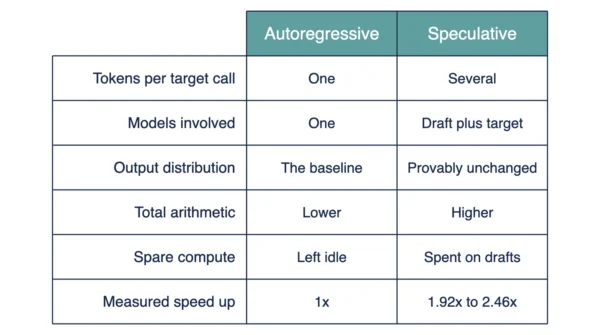
The table below sets the two decoding modes side by side, row by row. Every value traces back to the two papers named above.
| Aspect | Autoregressive decoding | Speculative decoding |
|---|---|---|
| What each paper calls it | Autoregressive sampling, namely ArS, per Chen | Speculative decoding (Leviathan) or speculative sampling, SpS (Chen) |
| Tokens per target-model forward pass | Still one token, always | Several tokens, capped by the draft length plus one |
| Serial calls needed to reach length L | L calls, one per token | Fewer calls, since each accepted draft token saves one serial call |
| Models involved | One, the target model alone | Two, namely a small draft model plus the target model |
| What the small model does | Not used at all | Drafts candidate tokens on its own, ahead of the target |
| What the big model does | Generates every token itself | Scores the whole draft in a single parallel pass, instead |
| How a wrong guess is handled | Not applicable, since nothing is guessed | Rejected by modified rejection sampling, then resampled from a corrected distribution |
| Effect on the output distribution | Still the baseline distribution itself | Unchanged, though: “the output distribution is guaranteed to remain unchanged” |
| Bit-identical outputs | Trivially so, by definition | Still not guaranteed in general; Chen: “we cannot not expect identical outputs” |
| Total arithmetic operations | Still the baseline amount | Higher, since rejected drafts waste computed work |
| Actual bottleneck | Namely memory bandwidth, per both papers | The same bottleneck, exploited rather than removed |
| What gets optimised | Neither, since this is the baseline case | Latency, still not total compute |
| Batch-size regime measured | Any batch size, generally | Batch size 1 in both papers, still a latency-first setting |
| Retraining or architecture change needed | Still not applicable | No, since Leviathan notes it works “without retraining or architecture changes” |
| Measured speedup | 1x, still the reference point in Chen’s Table 1 | “2X-3X” per Leviathan; a 2 to 2.5 times speedup for Chen, “without compromising the sample quality or making modifications to the model itself” |
| What governs the speedup | Raw model size and hardware bandwidth, generally | The acceptance rate between draft and target, also the draft model’s own cost |
| Where it is used today | Any autoregressive generation; still the default | Latency-critical serving, since a cheap same-family draft exists |
One row deserves a second look: bit-identical outputs. A guarantee about the distribution is not the same promise as identical text. The next section works through exactly why.
Why the Output Distribution Does Not Change
A common objection says speculative decoding must be an approximation, and every approximation trades some quality for speed. That objection is wrong for this specific method.
Leviathan and colleagues built it to run “without changing the distribution”. Later in the paper they state the result more forcefully: “A strong property of Algorithm 1 is that the output distribution is guaranteed to remain unchanged”. Chen and colleagues, working independently, reach the same conclusion through a different proof. Their scheme is “a novel modified rejection sampling scheme which preserves the distribution of the target model within hardware numerics”.
Leviathan illustrates the guarantee on a small unconditional-generation setup, where a 6M-parameter approximation model drafts for a 97M-parameter target model. Fewer serial calls are needed there too, while “the probability of generating it is unchanged”.
Distribution-identical, though, is a narrower promise than output-identical, and this is where most explanations of the method stop too early. Chen states the reason plainly: “because the different computation graphs lead to different numerics, we cannot not expect identical outputs”. That doubled “not” is the paper’s own wording, left exactly as printed.
Leviathan’s own results run the other way, inside their specific setup. Their abstract reports a “2X-3X” acceleration compared to the standard T5X implementation, “with identical outputs”. That claim holds for their argmax sampling on T5X. It is a property of that particular setting, not a universal law about the method.
Read the guarantee carefully, then. The output distribution is provably unchanged, in both papers, under two separate formal arguments. Bit-for-bit identical text is a stronger, narrower claim. It holds true in Leviathan’s argmax experiment. Chen’s own paper does not let you assume it in general.
It Does More Arithmetic, Not Less
Speculative decoding gets described, often, as a way to do less work. That description gets the trade backward. Leviathan devotes an entire section, titled Number of Arithmetic Operations, to the opposite finding.
Algorithm 1 runs several candidate continuations through the target model in parallel. That means “the number of concurrent arithmetic operations grows by a factor of” gamma plus one. When a drafted token gets rejected, the computation spent producing it is simply wasted. Total arithmetic rises. It does not fall.
Why does the method still make replies faster, if it burns more compute? Because arithmetic was never the actual constraint. Leviathan explains that large-model inference is “not bottlenecked on arithmetic operations, but rather on memory bandwidth and communication”. Chen states the same idea for their own setup: “Transformer sampling is typically memory bandwidth bound”.
Spare compute sits idle during ordinary decoding, precisely because ordinary decoding is not compute bound. Spending that spare compute to remove serial steps is a good trade, even while it burns more total FLOPs. Chen puts the payoff sharply: “the mean tokens per second with SpS often exceeds the idealised ceiling on auto-regressive sampling speed imposed by the memory bandwidth”.
That last line is worth sitting with. A method beats a ceiling that only exists for one-token-at-a-time decoding, by refusing to decode one token at a time.
What the Measured Speedups Actually Were
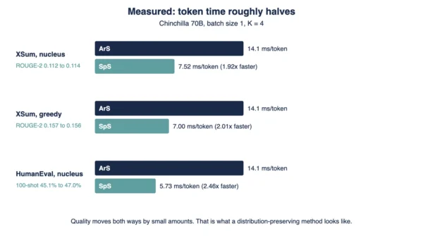
Chen and colleagues ran their headline comparison on Chinchilla, a 70B-parameter model, at batch size 1 with K = 4. XSum used nucleus sampling with p = 0.8, the same nucleus-versus-temperature choice our temperature vs top-p guide covers. HumanEval used p = 0.95 and a temperature of 0.8.
| Sampling method | Benchmark | Result | Mean token time | Speed up |
|---|---|---|---|---|
| ArS (Nucleus) | XSum (ROUGE-2) | 0.112 | 14.1ms/Token | 1x |
| SpS (Nucleus) | XSum (ROUGE-2) | 0.114 | 7.52ms/Token | 1.92x |
| ArS (Greedy) | XSum (ROUGE-2) | 0.157 | 14.1ms/Token | 1x |
| SpS (Greedy) | XSum (ROUGE-2) | 0.156 | 7.00ms/Token | 2.01x |
| ArS (Nucleus) | HumanEval (100 Shot) | 45.1% | 14.1ms/Token | 1x |
| SpS (Nucleus) | HumanEval (100 Shot) | 47.0% | 5.73ms/Token | 2.46x |
Read the mean-token-time column first, since that is the whole story here. Time per token drops by close to half across every row. Speculative sampling does the same job as autoregressive sampling, only faster.
Now read the Result column, carefully. HumanEval moves from 45.1% under autoregressive sampling to 47.0% under speculative sampling. XSum’s greedy ROUGE-2 moves the other way, from 0.157 down to 0.156. Neither movement is a quality change. The method is proven distribution-preserving. A higher or lower score on any single run is sampling variance, not a genuine gain and not a genuine loss.
XSum’s nucleus ROUGE-2 barely moves either, sliding from 0.112 to 0.114. Small movements in both directions, across every metric, are exactly what a distribution-preserving method should produce. A real quality change would need a different theoretical story, and neither paper tells one.
When It Does Not Help
Marketing language around speculative decoding often promises a flat two-to-three-times speedup. The papers themselves are more careful, and the condition list is short but firm.
Firstly, spare compute needs to be available. Leviathan is explicit that “speculative execution in general, and our algorithm in particular, assume that we have enough compute resources to support the increased concurrency”. Without that headroom, the extra parallel work has nowhere to run for free.
Secondly, the win depends on the acceptance rate. That is how often the draft model’s guess matches what the target model would have produced alone. A low acceptance rate means most drafted tokens get thrown away, and thrown-away work buys nothing.
Thirdly, the draft model itself has to stay cheap. Leviathan compared three approximation models against an 11B target: T5-large (800M), T5-base (250M) and T5-small (77M). The smallest one won: “T5-small (77M), with a good balance of c and” alpha, “provides the highest speedup out of the tested approximation models”. The largest draft model was not the fastest choice.
Finally, more draft tokens are not automatically better. A longer draft means fewer calls to the target model. It also means a longer loop each round, with a lower chance that every drafted token gets accepted.
Scope one more thing before trusting any of these numbers: every measurement here used batch size 1. That is a latency-first setting, not a throughput benchmark. Chen makes a related point about other techniques. They are “most effective at maximising throughout” (the paper’s own spelling) “(at larger batch sizes) instead of latency”. Treat the reported speedups as latency numbers, not general throughput claims.
Which One You Meet in Practice
Most systems you will actually touch are plain autoregressive decoders. That remains the default almost everywhere, and it likely stays that way for smaller deployments.
Speculative decoding shows up specifically where latency matters and a cheap same-family draft model already exists. Chat interfaces, code assistants and other single-user settings fit that profile well. Batch size 1 is exactly where both papers measured their gains.
Model size decides who gets to act as the draft, and target model size complicates that choice further. A Mixture of Experts target changes the calculus again. Our Mixture of Experts vs dense models guide explains why. Routing adds its own cost on top of the serial-step problem.
Speculative decoding is not the only lever for inference cost, either. Chen notes plainly that “this method can be used in conjunction many other techniques for accelerating or optimising the memory use of sampling”. Quantisation and multi-query attention are the two named examples. Our quantization vs distillation guide covers two of the levers teams often reach for instead.
For an exam or interview answer, lead with the mechanism rather than the headline number. Say which model drafts, say which model checks, and say what happens to a rejected guess. Those three facts separate the two approaches faster than any speedup figure.
Interview Questions
Frequently Asked Questions
Wrapping Up
The two decoding modes differ in shape, not in what they are allowed to produce. Autoregressive decoding runs one serial pass per token. Speculative decoding drafts ahead, then verifies in parallel.
Keep three facts from the papers, past the headline speedup number. The output distribution is provably unchanged, in both proofs, though bit-identical text is a narrower, setup-specific claim. Total arithmetic goes up, not down. Latency falls only because memory bandwidth, not arithmetic, was the actual limit all along.
Related reading on DiffStudy:
- Diffusion LLM vs Autoregressive
- Temperature vs Top-P
- Quantization vs Distillation
- Mixture of Experts vs Dense Models
- BERT vs GPT