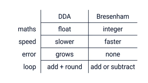
Overall, DDA vs Bresenham comes down to one thing: how each finds the next pixel. DDA uses floating-point maths, while Bresenham uses only integers. DDA computes an increment, then adds it and rounds at every step. Instead, Bresenham tracks a decision parameter and adds or subtracts small integers each step. Because Bresenham avoids division, rounding, and floating-point addition, it runs faster and never drifts off the true line. DDA is simpler to learn, so many courses teach it first. In practice, though, graphics libraries use Bresenham, or a close variant of it, for real pixel work.
Every line on a screen is really a row of pixels, since a screen has no room for perfectly smooth diagonals. So an algorithm must decide, pixel by pixel, which squares to light up. Indeed, DDA and Bresenham are the two classic answers to that problem.
GATE papers love this comparison, since examiners ask for the decision parameter, the pseudocode, or a worked line by hand. This guide walks through both algorithms in full. It also works one example line through each method, step by step, so you can check your own hand calculations against it.
Line drawing sits inside a bigger graphics pipeline. Clipping runs first, trimming lines to the visible window; read more on windowing and clipping in computer graphics for that earlier stage. When a line survives clipping, scan conversion turns it into pixels. That is exactly where DDA and Bresenham do their work.
What Line Drawing Actually Does
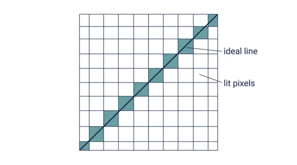
A mathematical line is continuous, since it has infinite points between its two ends. A screen, however, is a grid of discrete pixels. So nothing continuous survives contact with that grid unchanged.
Scan conversion is the process that bridges the two. It takes a line’s equation and picks the pixels that best approximate it. Every pixel sits at an integer coordinate. So the algorithm must round each computed point to its nearest integer position.
Rounding is unavoidable because a line’s true path rarely lands exactly on a pixel centre. Except at special slopes, such as exactly horizontal, vertical, or 45 degrees, the ideal line keeps crossing between pixels. Each algorithm must therefore choose the nearest pixel at every step. In short, that single choice, repeated many times, is the whole problem line drawing solves.
DDA and Bresenham both solve it. They just reach the same rounded pixel through very different arithmetic, as the worked example further down shows.
The DDA Algorithm
DDA stands for Digital Differential Analyzer. It is an incremental algorithm, so it builds the line one small step at a time. At each step, it adds a fixed increment to the previous point.
The steps are straightforward:
- Compute dx = x2 − x1 and dy = y2 − y1.
- Take steps = max(|dx|, |dy|), the larger of the two spans.
- Compute the increments: xIncrement = dx / steps and yIncrement = dy / steps.
- Start at (x1, y1). Add the increments after every step.
- Round each accumulated coordinate to the nearest integer. That rounded pair is the pixel to plot.
Here is the pseudocode:
dx = x2 - x1
dy = y2 - y1
steps = max(abs(dx), abs(dy))
xInc = dx / steps
yInc = dy / steps
x, y = x1, y1
plot(round(x), round(y))
for i in range(steps):
    x = x + xInc
    y = y + yInc
    plot(round(x), round(y))
Advantages of DDA:
- Simple to understand and to code, so it is often taught first.
- Works for any slope, since it always steps along the larger span.
- Needs only a handful of variables to track state.
Disadvantages of DDA:
- Needs floating-point arithmetic. It divides just to compute the increments.
- Rounds at every step, so small errors keep entering the calculation.
- Round-off error accumulates over long lines, and the pixel path can drift.
- Floating-point addition and rounding run slower than plain integer operations.
For the broader idea of writing steps like these before you code them, see the difference between an algorithm and a flowchart.
Bresenham’s Line Algorithm
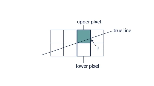
Bresenham’s algorithm answers the same question with only integers. Instead of a floating-point coordinate, it tracks a decision parameter. In fact, that parameter’s sign alone tells it which pixel comes next.
This walkthrough assumes a slope between 0 and 1, so dx is positive and larger than dy. For steeper lines, swap the roles of x and y, and step along y instead.
- Compute dx and dy, as before.
- Compute the initial decision parameter: p0 = 2·dy − dx.
- At each step, move x forward by one.
- If pk < 0, the next pixel is (xk+1, yk). Update pk+1 = pk + 2·dy.
- If pk ≥ 0, the next pixel is (xk+1, yk+1). Update pk+1 = pk + 2·dy − 2·dx.
- Repeat until x reaches x2.
Here is the pseudocode:
dx = x2 - x1
dy = y2 - y1
p = 2 * dy - dx
x, y = x1, y1
plot(x, y)
for i in range(dx):
    x = x + 1
    if p < 0:
        p = p + 2 * dy
    else:
        y = y + 1
        p = p + 2 * dy - 2 * dx
    plot(x, y)
Advantages of Bresenham’s algorithm:
- Uses only integer addition, subtraction, and a multiply by two, which is a bit shift.
- Needs no division and no rounding anywhere in the loop.
- Always picks the pixel closest to the true line, so accuracy stays high.
- Extends naturally to the midpoint circle algorithm.
- Maps well onto graphics hardware, since integer operations are cheap there.
Disadvantages of Bresenham’s algorithm:
- Needs a separate case for steep slopes, where x and y swap roles.
- Reads less intuitively than DDA at first, since the decision parameter takes some getting used to.
- Handles straight lines and circles, but free-form curves need different algorithms, such as Bezier or spline methods.
DDA vs Bresenham: Comparison Table
| Aspect | DDA | Bresenham |
|---|---|---|
| Arithmetic type | Floating-point | Integer only |
| Operations in the inner loop | Add, then round | Add or subtract, then compare |
| Division required | Yes, to compute the increments | No |
| Rounding required | Yes, at every step | No |
| Speed | Slower, due to floating-point work | Faster, integer work only |
| Accumulated error on long lines | Grows, from repeated rounding | None; steps stay exact integers |
| Accuracy of pixel choice | Approximate, rounded each step | Always the nearest pixel to the line |
| Decision variable | None; uses raw coordinates directly | Decision parameter p, updated each step |
| Implementation difficulty | Easier to learn and derive first | Slightly harder to follow at first |
| Hardware suitability | Poor fit for simple integer ALUs | Strong fit; maps onto shift-and-add logic |
| Extension to circles | Not the standard base for circles | Extends directly to the midpoint circle algorithm |
| Memory and register use | Needs floating-point registers | Needs only integer registers |
| Precision on long lines | Degrades as line length grows | Stays exact, regardless of length |
| Use in modern graphics libraries | Rare in production rasterisers | Common; still underpins many rasterisers |
Worked Example: The Same Line, Both Ways
Take the line from (2, 3) to (10, 8). Here dx = 8 and dy = 5, so the slope m = 0.625. Both algorithms plot the same starting pixel, (2, 3), before their loops even begin.
DDA: steps = 8, xIncrement = 1, and yIncrement = 0.625. The table below shows y accumulating, then rounding to a pixel at each step.
| Step k | x | y (accumulated) | Rounded pixel |
|---|---|---|---|
| 0 | 2 | 3.000 | (2, 3) |
| 1 | 3 | 3.625 | (3, 4) |
| 2 | 4 | 4.250 | (4, 4) |
| 3 | 5 | 4.875 | (5, 5) |
| 4 | 6 | 5.500 | (6, 6) |
| 5 | 7 | 6.125 | (7, 6) |
| 6 | 8 | 6.750 | (8, 7) |
| 7 | 9 | 7.375 | (9, 7) |
| 8 | 10 | 8.000 | (10, 8) |
Bresenham: p0 = 2(5) − 8 = 2. From here, only integer addition and subtraction decide each pixel.
| Step k | pk | Decision | Pixel plotted | pk+1 |
|---|---|---|---|---|
| 0 | 2 | pk ≥ 0 | (3, 4) | −4 |
| 1 | −4 | pk < 0 | (4, 4) | 6 |
| 2 | 6 | pk ≥ 0 | (5, 5) | 0 |
| 3 | 0 | pk ≥ 0 | (6, 6) | −6 |
| 4 | −6 | pk < 0 | (7, 6) | 4 |
| 5 | 4 | pk ≥ 0 | (8, 7) | −2 |
| 6 | −2 | pk < 0 | (9, 7) | 8 |
| 7 | 8 | pk ≥ 0 | (10, 8) | 2 |
Look closely at the final pixel lists. Both give (2,3), (3,4), (4,4), (5,5), (6,6), (7,6), (8,7), (9,7), (10,8), the same nine pixels either way. However, DDA needed floating-point addition and a rounding step at every point. In contrast, Bresenham needed only integer addition and subtraction. That one contrast is the entire argument between them.
Why Integer Arithmetic Wins
Processors handle integers faster than floating-point numbers, especially on simple or embedded hardware. Integer addition, subtraction, and bit shifts are cheap. Floating-point division and rounding cost more, both in time and in circuitry.
Bresenham’s inner loop needs only a compare, an add, and occasionally a subtract. Multiplying by two is just a left shift, not real multiplication. So every step of the loop maps directly onto basic integer hardware. This matters even for how a display refreshes; see how horizontal retrace and vertical retrace work if you want the full picture of how pixels reach the screen.
DDA’s inner loop, in contrast, needs a floating-point add and a round at every step. Rounding is not free, since it usually means a conversion step between floating-point and integer formats. Multiply that small cost by millions of pixels, and the gap becomes real.
Both algorithms are still O(n) in the number of pixels plotted, so their growth rate is identical; see our guide on time complexity if that idea needs a refresher. Even so, Bresenham simply carries a much smaller constant factor per step. Overall, that smaller constant, multiplied across an entire frame, is why it wins in practice.
Code Example
Below is a working Python version of both algorithms. Each returns the full list of plotted pixels, so you can run it and check the output against the worked example above.
def dda_line(x1, y1, x2, y2):
    dx = x2 - x1
    dy = y2 - y1
    steps = max(abs(dx), abs(dy))
    x_inc = dx / steps
    y_inc = dy / steps
    x, y = x1, y1
    pixels = [(round(x), round(y))]
    for _ in range(steps):
        x += x_inc
        y += y_inc
        pixels.append((round(x), round(y)))
    return pixels


def bresenham_line(x1, y1, x2, y2):
    dx = x2 - x1
    dy = y2 - y1
    p = 2 * dy - dx
    x, y = x1, y1
    pixels = [(x, y)]
    for _ in range(dx):
        x += 1
        if p < 0:
            p += 2 * dy
        else:
            y += 1
            p += 2 * dy - 2 * dx
        pixels.append((x, y))
    return pixels


print("DDA:", dda_line(2, 3, 10, 8))
print("Bresenham:", bresenham_line(2, 3, 10, 8))

# DDA: [(2, 3), (3, 4), (4, 4), (5, 5), (6, 6), (7, 6), (8, 7), (9, 7), (10, 8)]
# Bresenham: [(2, 3), (3, 4), (4, 4), (5, 5), (6, 6), (7, 6), (8, 7), (9, 7), (10, 8)]
Run this, and both functions return the same list of nine pixels. Notice that dda_line divides and calls round() at every step. Meanwhile, bresenham_line only ever adds, subtracts, and compares. Overall, that difference in the source code is the whole lesson in one glance.
When to Use Which
Use DDA when you are learning scan conversion for the first time, since its floating-point steps make the underlying idea easy to see. It also works fine for short lines or one-off tools, where speed barely matters.
Use Bresenham for anything resembling production graphics work. Rasterisers, low-level drivers, embedded displays, and plotting hardware all favour it, since integer speed and exact pixels matter there. Once pixels are chosen, they still need mapping into the final display region; see viewport vs window in computer graphics for how that mapping works. Overall, reach for Bresenham whenever performance or precision genuinely counts.
Interview Questions
Frequently Asked Questions
Wrapping Up
DDA and Bresenham both turn a mathematical line into a set of lit pixels. DDA does it with floating-point increments and a rounding step at every point. Meanwhile, Bresenham does it with an integer decision parameter, updated by addition and subtraction alone.
Remember the essentials for your exam. Both are incremental, though only DDA rounds inside its loop. Bresenham always picks the nearest pixel and never accumulates round-off error, so it wins on speed and on precision alike. When it is time to write real graphics code, Bresenham is almost always the right default.
Related reading on DiffStudy:
- Windowing vs Clipping in Computer Graphics
- Viewport vs Window in Computer Graphics
- Geometric Transformation vs Coordinate Transformation
- Horizontal Retrace vs Vertical Retrace
- CS Fundamentals hub