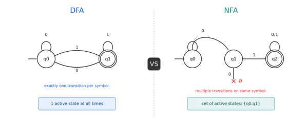
A DFA (Deterministic Finite Automaton) has exactly one transition per input symbol per state — predictable, easy to implement, preferred for compilers. An NFA (Nondeterministic Finite Automaton) can have multiple transitions or none for the same input — more flexible, fewer states, preferred for pattern matching. Every NFA can be converted to an equivalent DFA using the subset construction method. Both recognise exactly the same class of languages: regular languages.
In the debate of DFA vs NFA, both are essential finite state machines in automata theory and formal language theory — and both appear regularly in GATE, university exams, and technical interviews. While they recognise the same class of languages, they differ fundamentally in how they process input, how their transition functions are defined, and what trade-offs they offer in implementation. A DFA guarantees exactly one possible next state for every input symbol from every state. An NFA allows multiple possible next states, no transition at all, or spontaneous ε-transitions that consume no input. The practical consequence: NFAs are easier to design for complex patterns but harder to simulate; DFAs are harder to design but run in deterministic linear time. This guide covers formal definitions, state diagrams, a step-by-step NFA-to-DFA conversion, epsilon transitions, worked string processing examples, and GATE exam tips — everything you need to master both models.
Formal Definitions: The 5-Tuple Notation
Both DFA and NFA are formally defined as 5-tuples. This notation is mandatory for GATE and university exams — every question on automata theory assumes you know these definitions precisely.
DFA — Formal Definition
A DFA is defined as a 5-tuple:
- Q — Finite, non-empty set of states
- Σ — Finite set of input symbols (the alphabet)
- δ — Transition function: δ: Q × Σ → Q
Maps every (state, symbol) pair to exactly ONE next state - q₀ — The start state, where q₀ ∈ Q
- F — Set of accept states (final states), where F ⊆ Q
NFA — Formal Definition
An NFA is also defined as a 5-tuple:
- Q — Finite, non-empty set of states
- Σ — Finite set of input symbols (the alphabet)
- δ — Transition function: δ: Q × (Σ ∪ {ε}) → 2^Q
Maps every (state, symbol) pair to a SET of next states (including ∅) - q₀ — The start state, where q₀ ∈ Q
- F — Set of accept states (final states), where F ⊆ Q
The Critical Difference in the 5-Tuple
The structures look identical — but the transition function δ is fundamentally different. In a DFA, δ: Q × Σ → Q returns a single state. In an NFA, δ: Q × (Σ ∪ {ε}) → 2^Q returns a set of states (which can be empty, a singleton, or multiple states). This single change in the codomain of δ is what makes all the difference in behaviour, expressiveness, and implementation complexity.
Deterministic Finite Automaton (DFA)
A DFA is a finite state machine where for each state and each input symbol, there is exactly one transition defined. At any moment during processing, the machine is in precisely one state — no ambiguity, no parallelism. It processes input symbols left to right, one at a time, and after consuming all input, accepts the string if the current state is an accept state.
Example: DFA accepting strings ending in ‘1’ over Σ = {0, 1}
States: Q = {q0, q1}     Start: q0     Accept: {q1}

Transition Table:
┌────────┬──────────┬──────────┐
│ State  │ Input: 0 │ Input: 1 │
├────────┼──────────┼──────────┤
│  q0   │    q0    │    q1    │
│  q1   │    q0    │    q1    │
└────────┴──────────┴──────────┘

State diagram:
  ──→ (q0) ──1──→ ((q1))
       ↑ │             │
       └─┘ 0       0   │
       ←───────────────┘
       (q0 self-loop on 0, q1 self-loop on 1)

Processing "101": q0 →1→ q1 →0→ q0 →1→ q1 ✓ ACCEPT
Processing "110": q0 →1→ q1 →1→ q1 →0→ q0 ✗ REJECT
Advantages of DFA
- Deterministic execution: Exactly one computation path — always the same result for the same input
- Efficient simulation: O(n) time to process a string of length n — one state lookup per symbol
- Easy to implement: A single array or dictionary lookup per step — no backtracking or parallelism required
- Simpler to debug: Deterministic behaviour makes testing and verification straightforward
- Direct hardware implementation: DFAs map cleanly onto sequential circuits and tokenisers in compilers
Disadvantages of DFA
- State explosion: Converting an NFA with n states to a DFA can require up to 2ⁿ states (exponential blow-up in the worst case)
- Harder to design for complex patterns: Expressing languages like “strings containing ‘ab’ as a substring” requires more states in a DFA than in an equivalent NFA
- No epsilon transitions: Cannot take spontaneous transitions — every transition must consume an input symbol
- Total function requirement: Every (state, symbol) pair must have a defined transition — requiring a “dead state” (trap state) for undefined cases
Non-Deterministic Finite Automaton (NFA)
An NFA can have multiple transitions from one state on the same input symbol, no transition at all (which causes that path to die), or epsilon (ε) transitions that change state without consuming any input. The NFA is said to accept a string if at least one possible computation path leads to an accept state. Conceptually, the NFA explores all paths simultaneously — or equivalently, always “guesses” the right path.
Example: NFA accepting strings containing ’01’ as a substring over Σ = {0, 1}
States: Q = {q0, q1, q2}     Start: q0     Accept: {q2}

Transition Table:
┌────────┬───────────┬──────────┐
│ State  │ Input: 0  │ Input: 1 │
├────────┼───────────┼──────────┤
│  q0   │  {q0, q1} │  {q0}   │
│  q1   │    ∅      │  {q2}   │
│  q2   │  {q2}    │  {q2}   │
└────────┴───────────┴──────────┘

State diagram:
  ──→ (q0) ─0─→ (q1) ─1─→ ((q2))
       ↑↑                    ↑↑
      0,1 (self)            0,1 (self)

Processing "001":
  Start: {q0}
  Read 0: {q0, q1}   ← q0 loops, q0 also goes to q1
  Read 0: {q0, q1}   ← from q0→{q0,q1}, from q1→∅
  Read 1: {q0, q2}   ← from q0→{q0}, from q1→{q2}
  Final states include q2 (accept) ✓ ACCEPT
Advantages of NFA
- Fewer states: Can often represent a language with significantly fewer states than an equivalent DFA — important for constructing automata from regular expressions
- Easier to construct: Building an NFA directly from a regular expression (Thompson’s construction) is mechanical and produces compact automata
- Epsilon transitions: ε-transitions allow natural composition of automata — concatenation, union, and Kleene star are trivially implemented
- Regular expression engines: Most regex libraries internally build an NFA from the pattern — exploiting NFA’s compact representation
Disadvantages of NFA
- Harder to simulate directly: Must track all active states simultaneously (subset simulation) or use backtracking — more memory and complexity
- Non-deterministic execution: Cannot be directly implemented as a simple lookup table — requires set-based state tracking
- Harder to reason about: Multiple computation paths make manual tracing and debugging more complex
- Exponential DFA conversion: Converting an n-state NFA to a DFA can require up to 2ⁿ states — though in practice the actual DFA is often much smaller
Epsilon (ε) Transitions Explained
An epsilon (ε) transition is a transition in an NFA that moves from one state to another without consuming any input symbol. It represents a spontaneous state change — the machine can take the transition “for free.” Epsilon transitions do not exist in DFAs.
Example: NFA-ε accepting strings of the form aⁿ or bⁿ (only a’s or only b’s)
States: Q = {q0, q1, q2}     Start: q0     Accept: {q1, q2}

Transition Table (NFA-ε):
┌────────┬──────────┬──────────┬──────────┐
│ State  │ Input: a │ Input: b │  ε       │
├────────┼──────────┼──────────┼──────────┤
│  q0   │    ∅     │    ∅     │ {q1, q2} │
│  q1   │  {q1}   │    ∅     │    ∅     │
│  q2   │    ∅     │  {q2}   │    ∅     │
└────────┴──────────┴──────────┴──────────┘

State diagram:
         ε ──→ (q1) ─a─→ (q1) [self-loop]
              ↗
  ──→ (q0)
              ↘
         ε ──→ (q2) ─b─→ (q2) [self-loop]
Epsilon Closure (ε-closure)
The ε-closure of a state q is the set of all states reachable from q by following zero or more ε-transitions. It is essential for simulating NFA-ε and for converting NFA-ε to DFA.
For the example above:
  ε-closure(q0) = {q0, q1, q2}  ← q0 can reach q1 and q2 via ε
  ε-closure(q1) = {q1}           ← q1 has no ε-transitions
  ε-closure(q2) = {q2}           ← q2 has no ε-transitions

Processing "aaa":
  Start: ε-closure(q0) = {q0, q1, q2}
  Read a: δ({q0,q1,q2}, a) → from q1 only → {q1} → ε-closure = {q1}
  Read a: δ({q1}, a) → {q1} → ε-closure = {q1}
  Read a: δ({q1}, a) → {q1} → ε-closure = {q1}
  q1 ∈ F ✓ ACCEPT

Processing "ab":
  Start: ε-closure(q0) = {q0, q1, q2}
  Read a: → {q1}
  Read b: δ({q1}, b) → ∅ → ε-closure = ∅
  No accept state reachable ✗ REJECT
Why ε-transitions matter
Epsilon transitions make NFA construction modular. To build an NFA for the regular expression (a|b)*ab, you can independently build NFAs for a, b, and ab, then connect them with ε-transitions. Without ε-transitions, this composition would require designing a single monolithic automaton. Thompson’s construction algorithm (used in almost all regex engines) relies entirely on ε-transitions to compose larger NFAs from smaller ones.
Worked Example: Processing the Same String in DFA and NFA
The clearest way to see the difference is to process the same input string through both an equivalent DFA and NFA step by step. Below, both automata accept the language of strings over {0, 1} that end in ‘1’.
DFA — Processing “0101”
DFA: Q={q0,q1}, Accept={q1}, δ as above
Step  Symbol  Current → Next
  1     0      q0  →  q0
  2     1      q0  →  q1
  3     0      q1  →  q0
  4     1      q0  →  q1

Final state: q1 ∈ F  ✓ ACCEPT

At each step: exactly ONE next state.
No choices, no branching.
One linear path through the machine.
NFA — Processing “0101”
NFA (equivalent): same language, may differ in states
Step  Symbol  Active states → Next states
  1     0      {q0}  →  {q0}
  2     1      {q0}  →  {q0, q1}
  3     0      {q0,q1} → {q0}
               (q1 has no '0' transition)
  4     1      {q0}  →  {q0, q1}

Final states: {q0, q1}
q1 ∈ F  ✓ ACCEPT (at least one accept state)

At each step: a SET of active states.
Multiple parallel paths tracked simultaneously.
The Key Insight from This Example
The DFA has exactly one active state at all times — the machine is in one definite configuration. The NFA has a set of active states — it is simultaneously exploring multiple computation paths. The NFA accepts if any of its active states at the end of input is an accept state. In practice, simulating an NFA means tracking this set of active states, which is exactly what subset construction formalises into a DFA.
DFA vs NFA: 12 Critical Differences
Aspect | DFA | NFA |
|---|---|---|
| Transition function | δ: Q × Σ → Q — returns exactly one state | δ: Q × (Σ ∪ {ε}) → 2^Q — returns a set of states |
| Active states at any time | Exactly one state — fully deterministic configuration | A set of states — multiple parallel paths explored simultaneously |
| Epsilon (ε) transitions | Not allowed — every transition must consume an input symbol | Allowed — machine can change state without consuming any input |
| Undefined transitions | Not allowed — δ must be defined for every (state, symbol) pair; undefined cases use a dead (trap) state | Allowed — δ may return ∅ (empty set) meaning that computation path dies |
| Acceptance condition | Accepts if the single final state is in F after all input is consumed | Accepts if at least one state in the final set of active states belongs to F |
| Number of states | Can require exponentially more states (up to 2ⁿ) than an equivalent NFA | Can represent many languages with fewer states than the equivalent DFA |
| Ease of construction | Harder to design from scratch for complex patterns — requires careful state planning | Easier to build — can be constructed directly from regular expressions using Thompson’s construction |
| Simulation complexity | O(n) time, O(1) space — one lookup per symbol, one current state to track | O(n × |Q|) time in subset simulation — must track the entire set of active states per step |
| Conversion | Every DFA is trivially an NFA (single-state sets as transition outputs) | Every NFA can be converted to an equivalent DFA using subset construction — but may cause state explosion |
| Expressive power | Recognises exactly the class of regular languages | Recognises exactly the class of regular languages — same power, different representation efficiency |
| Primary use case | Lexical analysis (tokenisation) in compilers; pattern matching in performance-critical systems | Regular expression engines; Thompson’s construction; theoretical analysis and language proofs |
| Backtracking | No backtracking — single deterministic path, no dead ends to recover from | No backtracking needed if simulated with subset construction — all paths tracked simultaneously |
NFA to DFA Conversion: Subset Construction Method
Every NFA can be converted to an equivalent DFA that accepts exactly the same language. The algorithm is called subset construction (or the powerset construction). The core idea: each state of the DFA corresponds to a set of NFA states that the NFA could be in simultaneously.
Why This Works
When simulating an NFA, we track a set of active states at each step. Subset construction turns each such set into a single DFA state. An n-state NFA can produce at most 2ⁿ DFA states (one per subset of Q), but in practice most subsets are unreachable and the actual DFA is much smaller.
Step-by-Step Conversion: Worked Example
Given NFA: Accepts strings over {a, b} containing ‘ab’ as a substring.
NFA States: Q = {q0, q1, q2}
Alphabet: Σ = {a, b}
Start: q0     Accept: {q2}

NFA Transition Table:
┌────────┬───────────┬──────────┐
│ State  │    a      │    b     │
├────────┼───────────┼──────────┤
│  q0   │ {q0, q1}  │  {q0}   │
│  q1   │    ∅      │  {q2}   │
│  q2   │  {q2}    │  {q2}   │
└────────┴───────────┴──────────┘
Step 1: Start with the ε-closure of the NFA start state. (No ε-transitions here, so ε-closure(q0) = {q0}.)
DFA start state = A = {q0}
Step 2: For each DFA state (set of NFA states), compute transitions on each input symbol by applying δ to every NFA state in the set and taking the union.
DFA State    On 'a'                          On 'b'
─────────────────────────────────────────────────────
A = {q0}     δ(q0,a) = {q0,q1} → B          δ(q0,b) = {q0} → A
B = {q0,q1}  δ(q0,a)∪δ(q1,a) = {q0,q1}∪∅   δ(q0,b)∪δ(q1,b) = {q0}∪{q2}
             = {q0,q1} → B                  = {q0,q2} → C
C = {q0,q2}  δ(q0,a)∪δ(q2,a) = {q0,q1}∪{q2} δ(q0,b)∪δ(q2,b) = {q0}∪{q2}
             = {q0,q1,q2} → D               = {q0,q2} → C
D={q0,q1,q2} δ(q0,a)∪δ(q1,a)∪δ(q2,a)      δ(q0,b)∪δ(q1,b)∪δ(q2,b)
             = {q0,q1}∪∅∪{q2} = {q0,q1,q2} = {q0}∪{q2}∪{q2}
             → D                             = {q0,q2} → C
Step 3: Mark accept states. Any DFA state whose NFA subset contains an NFA accept state (q2) is a DFA accept state.
Final DFA:
┌──────────────────┬──────┬──────┬──────────┐
│ DFA State        │  a   │  b   │ Accept?  │
├──────────────────┼──────┼──────┼──────────┤
│ A = {q0}    →   │  B   │  A   │   No     │
│ B = {q0,q1} →   │  B   │  C   │   No     │
│ C = {q0,q2} →   │  D   │  C   │  YES ✓   │
│ D={q0,q1,q2}→   │  D   │  C   │  YES ✓   │
└──────────────────┴──────┴──────┴──────────┘

DFA has 4 states. NFA had 3 states.
(State explosion avoided here — worst case would be 2³ = 8 states)
Step 4: Verify. Processing “ab” in the DFA: A →a→ B →b→ C (accept ✓). Processing “ba”: A →b→ A →a→ B (reject ✓, ‘ba’ doesn’t contain ‘ab’). The converted DFA is correct.
General Subset Construction Algorithm
- Compute ε-closure(q₀) — this is the DFA start state. Add to an unmarked worklist.
- While there are unmarked DFA states in the worklist:
- Mark the current DFA state S (a set of NFA states)
- For each input symbol a ∈ Σ: compute T = ε-closure(δ(S, a)) = ε-closure( ∪_{q∈S} δ(q, a) )
- If T is not already a DFA state, add it to the worklist (unmarked)
- Add transition: DFA δ(S, a) = T
- Any DFA state S where S ∩ F ≠ ∅ (S contains an NFA accept state) is a DFA accept state.
- The DFA has at most 2^|Q| states — but unreachable subsets are never generated, so the practical DFA is usually much smaller.
Python Implementation
DFA Implementation
class DFA:
    def __init__(self, transitions,
                 start_state, accept_states):
        self.transitions = transitions
        self.start = start_state
        self.accept = accept_states

    def process(self, input_string):
        state = self.start
        for char in input_string:
            state = self.transitions.get(
                (state, char))
            if state is None:
                return False  # dead state
        return state in self.accept

# DFA accepting strings ending in '1'
dfa = DFA(
    transitions={
        ('q0','0'):'q0', ('q0','1'):'q1',
        ('q1','0'):'q0', ('q1','1'):'q1'
    },
    start_state='q0',
    accept_states={'q1'}
)
print(dfa.process('101'))  # True
print(dfa.process('110'))  # False
NFA Implementation (Subset Simulation)
class NFA:
    def __init__(self, transitions,
                 start_state, accept_states):
        self.transitions = transitions
        self.start = start_state
        self.accept = accept_states

    def process(self, input_string):
        # Track SET of active states
        active = {self.start}
        for char in input_string:
            next_states = set()
            for state in active:
                next_states.update(
                    self.transitions.get(
                        (state, char), set()))
            active = next_states
        # Accept if any active state is final
        return bool(active & self.accept)

# NFA accepting strings containing 'ab'
nfa = NFA(
    transitions={
        ('q0','a'):{'q0','q1'},
        ('q0','b'):{'q0'},
        ('q1','b'):{'q2'},
        ('q2','a'):{'q2'},
        ('q2','b'):{'q2'}
    },
    start_state='q0',
    accept_states={'q2'}
)
print(nfa.process('ab'))   # True
print(nfa.process('bab'))  # True
print(nfa.process('ba'))   # False
Best Practices for Implementation:
Use dictionaries for O(1) transition lookups. For NFA simulation, represent active states as a Python set — set union and intersection operations are efficient and semantically correct. When implementing subset construction, use a dictionary keyed by frozensets (since sets are unhashable) to represent DFA states. Always test with strings both inside and outside the target language, and test boundary cases: the empty string ε, single-character strings, and strings that partially match the pattern.
GATE Exam Tips: DFA vs NFA
Important for GATE, UGC-NET, and University Exams
DFA vs NFA is a consistently tested topic in GATE CS. Questions typically test: formal definitions, state minimisation, conversion, equivalence proofs, and language recognition. The points below are the most frequently examined concepts.
Must-Know Facts for GATE
- ✅ Same expressive power: DFA ≡ NFA ≡ NFA-ε — all three recognise exactly the class of regular languages. This is Kleene’s theorem. Very frequently examined.
- ✅ State complexity: An NFA with n states may require up to 2ⁿ states in the equivalent DFA. But some languages require exactly this — e.g., the language accepted by a specific n-state NFA can require 2ⁿ DFA states in the worst case.
- ✅ Every DFA is an NFA: A DFA is a special case of NFA where δ(q, a) is always a singleton set. The converse requires subset construction.
- ✅ Minimisation applies only to DFA: The algorithm for minimising the number of states (Myhill-Nerode, table-filling algorithm) applies to DFAs, not directly to NFAs.
- ✅ Dead state: In a complete DFA, undefined transitions go to a non-accept “dead state” (trap state) with self-loops on all inputs. In incomplete DFAs (allowed in some textbooks), undefined transitions implicitly reject.
- ✅ ε-closure: Must know how to compute ε-closure of a set of states — it is used in every NFA-to-DFA conversion question.
Common GATE Question Types
- 📝 Identify language accepted: Given a DFA/NFA transition table, determine the language it accepts — trace several strings to find the pattern
- 📝 Construct from language: “Design a DFA/NFA accepting all strings over {0,1} with an even number of 0s” — know how to design both types
- 📝 Minimum states: “What is the minimum number of states in a DFA accepting…?” — use Myhill-Nerode theorem or identify equivalence classes
- 📝 NFA to DFA conversion: Given an NFA, construct the equivalent DFA using subset construction — always shown as a full worked question
- 📝 Membership testing: “Does the DFA/NFA accept the string ‘w’?” — trace step by step and state which states are active at each step
- 📝 True/False statements: e.g., “Every NFA has an equivalent DFA” (True), “NFA can accept non-regular languages” (False), “Minimisation of NFA is always possible” (complex — be careful)
Quick Reference: Key Theorems and Results
| Theorem / Result | Statement | Exam Relevance |
|---|---|---|
| Rabin-Scott (1959) | Every NFA has an equivalent DFA (subset construction proves this) | Foundational — examiners test understanding, not just memorisation |
| State complexity bound | An NFA with n states → DFA with at most 2ⁿ states; tight bound exists | High — “minimum DFA states” questions appear every few years |
| DFA minimisation | For every DFA there is a unique minimum-state DFA (up to isomorphism) | Medium — table-filling algorithm questions appear occasionally |
| Closure properties | Regular languages are closed under union, intersection, complement, concatenation, Kleene star | High — proof questions using DFA/NFA constructions for each operation |
| Pumping Lemma | Used to prove a language is NOT regular (cannot be shown with DFA/NFA) | High — at least one pumping lemma question per GATE exam |
Frequently Asked Questions
re module, Perl regex, Java Pattern) because they are easier to construct from regex syntax using Thompson’s construction and often require fewer states. The engine either simulates the NFA directly using subset tracking, or converts it to a DFA first (DFA-based regex engines like RE2 and Hyperscan do this for guaranteed linear-time matching). NFAs also appear in natural language processing, network protocols, and formal verification.For example, in a DFA recognising the language {ab}, if the machine reads ‘b’ in the start state (expecting ‘a’ first), it enters a dead state and stays there regardless of subsequent input. In NFA transition tables, the equivalent is returning ∅ (the empty set) — that computation path simply dies rather than requiring an explicit dead state. Dead states add to the state count of a DFA but are important for theoretical completeness and for implementing the complement of a regular language (complement of a DFA is obtained by swapping accept and non-accept states — dead states must be included to get the correct complement).
Use Cases and Applications
Both DFA and NFA find applications in lexical analysis, pattern matching, parsing, and network protocols. DFA is commonly used in compilers for tokenisation and syntax analysis due to its deterministic, O(n) runtime, while NFA is employed in regular expression matching algorithms for its compact representation and ease of construction from patterns.
DFA — Key Takeaways:
- 5-tuple M = (Q, Σ, δ, q₀, F) where δ: Q × Σ → Q
- Exactly one active state at all times — fully deterministic
- No ε-transitions; complete transition function required
- O(n) time, O(1) space to process a string of length n
- May require up to 2ⁿ states vs equivalent NFA
- Best for: compilers, lexical analysers, hardware controllers
NFA — Key Takeaways:
- 5-tuple M = (Q, Σ, δ, q₀, F) where δ: Q × (Σ∪{ε}) → 2^Q
- Multiple active states simultaneously — tracks all paths
- ε-transitions allowed; transitions to ∅ allowed
- Accepts if any final active state ∈ F
- Often far fewer states than equivalent DFA
- Best for: regex engines, Thompson’s construction, theory proofs
Related Topics Worth Exploring
Mealy vs Moore Machine
DFA and NFA are recognisers — they accept or reject strings. Mealy and Moore machines are transducers — they produce output on each transition or in each state. Understanding the relationship between these four automata types completes the picture of finite state machine theory tested in GATE and university courses.
NP-Hard vs NP-Complete
Finite automata theory (DFA, NFA, regular languages) is the foundation of formal language theory. NP-Hard and NP-Complete problems sit at the other end of the Chomsky hierarchy — in the class of problems decidable by non-deterministic Turing machines in polynomial time. Understanding both ends of the hierarchy is essential for GATE Theory of Computation.
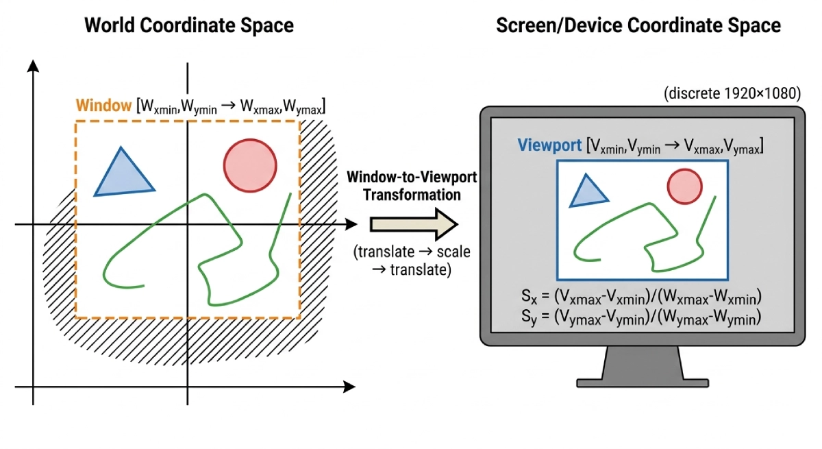
Windowing vs Clipping in Computer Graphics
The boundary-enforcement logic of clipping algorithms — where points outside a defined region are discarded — has a structural parallel to how DFA dead states and NFA empty-set transitions discard computation paths that fall outside the accepted language. Understanding both builds stronger intuition for boundary conditions in formal systems.