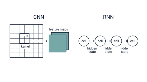
A CNN (Convolutional Neural Network) suits grid-like data, such as images. It slides small filters across the input and shares those weights across space. An RNN (Recurrent Neural Network) suits sequential data, such as text or time series. It steps through the sequence one element at a time. It carries a hidden state forward as memory, sharing weights across time instead of space. Since 2017, Transformers have taken over most large-scale NLP work from RNNs. CNNs, though, remain the default for vision. In short, pick a CNN for spatial data. Pick an RNN, or often now a Transformer, for sequential data.
Two architectures shaped deep learning before Transformers arrived. They are Convolutional Neural Networks (CNN) and Recurrent Neural Networks (RNN). Between them, these two models revolutionised computer vision, natural language processing, and speech recognition. This guide works through the core differences between CNN and RNN. You will come away with a clear picture of their strengths and their applications.
If you are new to the field, start with how deep learning fits inside machine learning. Both CNNs and RNNs, after all, are deep-learning models built from stacked layers.
The core question is simple: what shape does your data take? A CNN assumes the input is a grid, where nearby pixels relate to each other. An RNN assumes the input is a sequence, where order carries the meaning. This guide defines each architecture and shows how it processes data. It then compares the two in full. Along the way, it explains where Transformers fit and when each architecture still earns its place.
What is a CNN?
A Convolutional Neural Network, or ConvNet, is designed for grid-like data, such as images or 2D signals. It leans on convolutional layers to learn features automatically. Nobody needs to hand-craft those features first. Because it captures spatial relationships so well, a CNN excels at image classification, object detection, and image segmentation.
Its core building blocks are convolutional layers, pooling layers, and fully connected layers. Convolutional layers use filters, or kernels, for local receptive-field operations. Stacking several such layers builds a feature hierarchy. Early layers learn edges and textures. Later layers learn whole objects and patterns. Pooling layers, such as max or average pooling, then shrink the spatial dimensions of those features. This makes the network more robust to small shifts. Finally, fully connected layers consolidate everything the network has learned into a prediction.
Advantages of a CNN:
- Learns spatial feature hierarchies automatically. No manual feature engineering is needed.
- Shares filter weights across the whole input, so the parameter count stays low.
- Gains translation invariance from pooling, so small shifts barely change the output.
- Trains efficiently in parallel, since one convolution does not depend on another.
Disadvantages of a CNN:
- Expects a fixed-size input. Images usually need resizing or cropping first.
- Is not a natural fit for variable-length sequential data.
- Still needs a large labelled dataset. Training from scratch also takes real compute.
What is an RNN?
A Recurrent Neural Network is tailored for sequential data, where order matters. Unlike a CNN, an RNN has loops within its architecture. Those loops let it keep a memory of past inputs. That memory lets an RNN handle sequences of varying length. It also captures dependencies that stretch across time. As a result, RNNs do well at speech recognition, language translation, and sentiment analysis.
Because of those loops, an RNN is recurrent, not feedforward. Information flows in cycles, not just forward. The key part is the recurrent cell. It keeps a hidden state and takes two inputs: the current input and the previous hidden state. That hidden state acts as memory. It carries information from earlier inputs forward. This is what lets an RNN model sequences at all. Several cell variants exist: the simple RNN cell, the LSTM cell, and the GRU cell. These variants mainly help capture longer-term dependencies. They also ease the vanishing gradient problem common in deep networks.
Advantages of an RNN:
- Handles variable-length sequences naturally. A fixed-size network cannot do this.
- Shares the same cell weights at every timestep, so the parameter count does not grow with length.
- Captures long-range dependencies well, especially with LSTM or GRU cells.
- Suits streaming or online inference, where input can arrive one token at a time.
Disadvantages of an RNN:
- Computes sequentially. It cannot parallelise across timesteps the way a CNN parallelises across space.
- Can suffer from vanishing or exploding gradients on long sequences. LSTM and GRU cells only ease this; they do not remove it.
- Has been largely replaced by Transformers for large-scale NLP. It still matters in smaller or streaming settings.
CNN vs RNN: Comparison Table
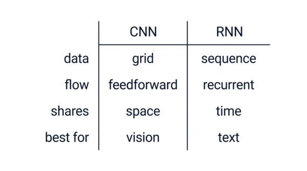
| Aspect | CNN | RNN |
|---|---|---|
| Architecture | Feedforward | Recurrent |
| Data type | Grid-like (images, 2D signals) | Sequential (text, speech, time series) |
| Memory | No explicit memory | Has memory via a hidden state for temporal dependencies |
| Processing | Local receptive-field convolutions | Sequential processing through recurrent connections |
| Parameter sharing | Shares filter weights across space | Shares cell weights across time |
| Strength | Spatial feature extraction | Temporal dependency modelling |
| Applications | Image classification, object detection, image segmentation | Language modelling, speech recognition, time series analysis |
| Training | Parallelisable, since convolutions are independent | Sequential, since each step depends on the last |
| Vanishing gradient | Not as prone to the problem | Can suffer from it, though LSTM/GRU cells ease it |
| Inputs | Fixed-size inputs | Variable-size inputs |
| Memory during training | Activations stored across the spatial feature map | Hidden states stored across timesteps (backpropagation through time) |
| Output pattern | Typically one label or map per input | Naturally sequence-to-sequence or sequence-to-one |
| Hardware fit | Convolutions map well onto parallel GPU/TPU cores | Per-step dependency limits parallel speed-up on the same hardware |
| Modern status | Still the default for vision, alongside Vision Transformers | Largely replaced by Transformers for large-scale NLP |
| Best for | Spatial data: photos, video frames, scans | Sequential data: text, audio, sensor streams |
How Each Processes Data
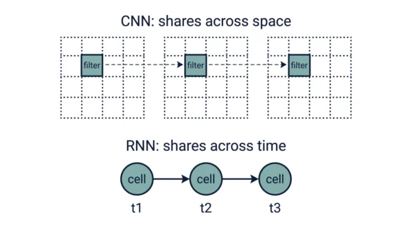
The cleanest way to see the difference is to watch each network handle input. Picture a CNN looking at a photo. It slides a small kernel, say 3×3 pixels, over the image. At each position, it computes one dot product and writes the result into a feature map. The same kernel weights get reused at every position. So a CNN shares its parameters across space. Stack several such layers, and the network builds a hierarchy. Early layers learn edges and textures. Later layers learn whole objects and patterns.
Now picture an RNN reading a sentence. It processes one word at a time. At each step, the recurrent cell takes the current word’s embedding and the previous hidden state. It then produces a new hidden state. The very same cell weights apply at every timestep. So an RNN shares its parameters across time instead of across space. That single design choice sums up the whole comparison. A CNN reuses one filter everywhere in the image. An RNN, instead, reuses one cell at every step in the sequence.
This step-by-step dependency also explains the hardware gap. Since each hidden state needs the one before it, a GPU cannot compute every timestep at once. It can, however, compute all the positions of one convolution at once. For more on real training hardware, see our comparison of GPUs, TPUs, and NPUs for AI workloads.
Applications
CNN applications span a wide range of vision tasks:
- Image classification: a CNN sorts images into categories with high accuracy. This enables autonomous driving, medical image analysis, and content-based image retrieval.
- Object detection: combined with bounding box regression and non-maximum suppression, a CNN finds and classifies objects in an image. This matters for video surveillance and self-driving cars.
- Image segmentation: a CNN can label every pixel in an image. This is crucial in medical imaging for tumour detection and organ segmentation.
RNN applications centre on sequential and temporal data:
- Language modelling: an RNN models the probability of a word sequence, so it can generate coherent, relevant text. This benefits translation, chatbots, and speech recognition.
- Speech recognition: an RNN, especially with LSTM or GRU cells, converts speech into text. It is widely used in voice assistants, transcription, and call centres.
- Time series analysis: an RNN models and predicts data over time. This suits stock forecasting, weather prediction, and anomaly detection.
Where Transformers Fit
No modern comparison of CNN and RNN is complete without the Transformer. It is the single biggest change to this picture since 2017. That year, the paper “Attention Is All You Need” introduced self-attention. This architecture drops recurrence entirely. Self-attention lets every position in a sequence look directly at every other position, in one step. It need not wait for information to travel forward one timestep at a time, the way an RNN must.
Because a Transformer has no step-by-step dependency, it trains in parallel across a whole sequence. That is dramatically faster on modern GPUs than an RNN’s forced timestep-by-timestep computation. Self-attention also tends to hold onto long-range dependencies better than a simple recurrent cell. For that reason, Transformers have largely replaced RNNs for large-scale translation, language modelling, and chatbots. This even includes the large language models behind today’s most capable NLP tools.
CNNs, by contrast, remain the default for most vision work. Vision Transformers, or ViTs, now compete with them on large image datasets. A ViT treats an image as a sequence of patches. Meanwhile, RNNs and LSTMs have not vanished. They still show up in small models, streaming applications, and some time-series forecasting tasks. A lighter, sequential design is often easier to run than full attention. So the honest summary is this: Transformers changed the default for sequence work. They did not make RNNs useless everywhere.
Code Example
The clearest way to see the shape difference is a minimal model of each. Both snippets below use Keras. Both are illustrative sketches of the layer shapes, not a trained or executed pipeline.
from tensorflow import keras
from tensorflow.keras import layers

# Minimal CNN: a batch of 28x28 grayscale images
cnn = keras.Sequential([
    layers.Input(shape=(28, 28, 1)),
    layers.Conv2D(32, kernel_size=3, activation="relu"),
    layers.MaxPooling2D(pool_size=2),
    layers.Flatten(),
    layers.Dense(10, activation="softmax"),
])

# Minimal RNN: a batch of 20-step sequences, 8 features per step
rnn = keras.Sequential([
    layers.Input(shape=(20, 8)),
    layers.LSTM(32),
    layers.Dense(10, activation="softmax"),
])
Notice what each input shape says about the data it expects. The CNN’s Input(shape=(28, 28, 1)) describes a 2D grid with one channel. Its Conv2D and MaxPooling2D layers work across that grid’s height and width. The RNN’s Input(shape=(20, 8)) instead describes 20 ordered timesteps. Its single LSTM layer walks through them one at a time. It then hands a summary to the final Dense layer. So even before training, the input shape alone tells you which architecture you are looking at.
When to Use Which
Choosing between a CNN and an RNN starts with a simple question: what shape does your data actually have?
Use a CNN whenever the input is naturally grid-shaped. Photographs, video frames, medical scans, and 3D sensor grids all qualify. Nearby positions relate to each other there. For very large vision datasets, a Vision Transformer is worth a look too. Still, a CNN remains the safer default for most projects.
Use an RNN, and specifically an LSTM or GRU, when the sequence is short to moderate. It also fits streaming or low-latency inference, or projects where compute and data are limited. However, once you work with large text corpora, or need strong long-range dependencies, a Transformer usually fits better. That is precisely because it trains in parallel and captures those dependencies more reliably.
Interview Questions
Frequently Asked Questions
Wrapping Up
CNN and RNN approach deep learning from two different directions. A CNN slides a shared filter across space. This pulls spatial features out of grid-like data. An RNN, in contrast, steps through a sequence. It shares one cell across time, carrying a hidden state forward as memory.
Remember the essentials. CNNs excel with grid-like data, such as images. RNNs, and their LSTM or GRU variants, excel with sequences where order matters. Since 2017, Transformers have taken over most large-scale sequence work. Self-attention trains in parallel, where recurrence cannot. Even so, the right choice always depends on your data and your task. Understanding CNN and RNN properly is still the fastest way to see why Transformers work as they do.
Related reading on DiffStudy:
- Machine Learning vs Deep Learning
- GPU vs TPU vs NPU for AI Workloads
- Retrieval-Augmented Generation vs Fine-Tuning
- CS Fundamentals hub