Algorithm analysis is the foundation of every engineering decision that matters at scale. In 2026, as software systems process petabytes of data and serve billions of users, understanding how an algorithm behaves under pressure is no longer optional — it is the difference between systems that thrive and systems that collapse. At the core of this analysis sits asymptotic notation: the mathematical language developers use to describe how algorithms grow. The three pillars of this language — Big O, Big Theta, and Big Omega notation — each tell a different part of the performance story. Big O describes the worst that can happen, Big Theta defines exactly what will happen, and Big Omega establishes the best possible outcome. Whether you are a student preparing for technical interviews, a developer optimizing production code, or an architect evaluating competing algorithms, mastering the distinctions between these three notations gives you the vocabulary and analytical framework to make rigorous performance decisions rather than educated guesses.
Asymptotic Notation in Algorithm Analysis
Every algorithm you write has a performance story. That story changes depending on the size of the input it receives. A sorting algorithm that handles 100 elements in milliseconds may take hours on a million-element dataset if its underlying complexity is poor. Asymptotic notation gives computer scientists and engineers a standardized, mathematically precise way to describe this behavior — specifically how running time or memory usage scales as input size approaches infinity.
The three primary asymptotic notations — Big O (O), Big Theta (Θ), and Big Omega (Ω) — were formalized by Donald Knuth in 1976, drawing on earlier mathematical work by Paul Bachmann and Edmund Landau. Each notation answers a different question about algorithmic performance. Together they form a complete picture, but in isolation each serves a distinct analytical purpose that practicing engineers must understand to apply them correctly.
A critical misconception worth addressing immediately: Big O notation does not exclusively describe worst-case performance. Big O describes an upper bound on a function’s growth rate. Worst-case, average-case, and best-case are separate analytical dimensions that each use whichever notation is most appropriate. An algorithm can have a worst-case complexity expressed as O(n²), a best-case expressed as Ω(n log n), and a tight bound for a specific case expressed as Θ(n). Understanding this distinction separates developers who use notation fluently from those who apply it mechanically.

Big O Notation: Upper Bound Deep Dive
Definition
Big O notation, written O(f(n)), provides an asymptotic upper bound on the growth rate of a function. Formally, a function T(n) is O(f(n)) if there exist positive constants c and n₀ such that T(n) ≤ c·f(n) for all n ≥ n₀. In plain terms, Big O says: “this function will never grow faster than f(n) beyond a certain input size.” It establishes a ceiling on behavior, making it the most widely used notation for communicating algorithm performance because it answers the question engineers most often need answered: “what is the worst I should expect from this algorithm as my data grows?”
Advantages
- Universal standard: Universally understood by developers, academics, and interviewers, making it the lingua franca of algorithm communication
- Worst-case safety: Guarantees performance ceiling, enabling capacity planning and SLA commitments with confidence
- Simplification power: Drops constants and lower-order terms, focusing attention on dominant growth behavior that matters at scale
- Comparison tool: Enables direct algorithm comparison across different implementations and languages
- Interview currency: The notation most expected and evaluated in technical interviews at every level from entry to staff engineer
Limitations
- Pessimistic by nature: Upper bound may be loose, describing behavior that never actually occurs in practice for many inputs
- Hides constants: O(100n) and O(n) are equivalent in Big O, but the 100x constant factor matters enormously in real systems
- No lower bound insight: Says nothing about how well an algorithm performs on favorable inputs
- Input distribution blind: Treats all input distributions identically, which misrepresents performance for algorithms with strong average-case behavior
- Asymptotic only: Describes behavior at large n; may mislead for small practical input sizes where lower-order terms dominate
Common Big O Complexities Ranked
| Notation | Name | Example Algorithm | n=1,000 Operations (approx) |
|---|---|---|---|
| O(1) | Constant | Array index access, hash table lookup | 1 |
| O(log n) | Logarithmic | Binary search, balanced BST operations | ~10 |
| O(n) | Linear | Linear search, single array traversal | 1,000 |
| O(n log n) | Linearithmic | Merge sort, heap sort, fast Fourier transform | ~10,000 |
| O(n²) | Quadratic | Bubble sort, insertion sort, naive matrix multiply | 1,000,000 |
| O(2ⁿ) | Exponential | Recursive Fibonacci, traveling salesman brute force | 2^1000 (astronomical) |
Formal Mathematical Definition:
T(n) = O(f(n)) if and only if there exist positive constants c and n₀ such that 0 ≤ T(n) ≤ c·f(n) for all n ≥ n₀. The notation captures the idea that beyond a threshold input size n₀, the function T(n) is always bounded above by some constant multiple of f(n). When we say an algorithm is O(n²), we are asserting that its running time will never exceed some constant times n² for sufficiently large inputs — regardless of what specific input triggers the worst case.
Big Theta Notation: Tight Bound Deep Dive
Definition
Big Theta notation, written Θ(f(n)), provides a tight asymptotic bound on a function’s growth rate, meaning it simultaneously establishes both an upper and lower boundary. Formally, T(n) is Θ(f(n)) if there exist positive constants c₁, c₂, and n₀ such that c₁·f(n) ≤ T(n) ≤ c₂·f(n) for all n ≥ n₀. In plain terms, Big Theta says: “this function grows at exactly the same rate as f(n), neither faster nor slower, beyond a certain input size.” If Big O is a ceiling and Big Omega is a floor, Big Theta is both simultaneously — the function is sandwiched between two constant multiples of f(n). Therefore, Θ provides the most precise characterization of an algorithm’s complexity when the upper and lower bounds coincide.
Advantages
- Maximum precision: Tells you exactly how the algorithm grows, not just a bound — the most informative single notation available
- No ambiguity: Eliminates the looseness of Big O by requiring both upper and lower bounds to match the same function
- Theoretical foundation: Preferred in academic literature and formal proofs where precision matters over convenience
- Bidirectional guarantee: Simultaneously promises the algorithm will never be worse than the bound and never better than the bound
- Optimality proofs: When an algorithm’s complexity matches a proven lower bound for a problem, Theta notation expresses that the algorithm is asymptotically optimal
Limitations
- Not always applicable: Many algorithms have different best and worst case complexities, making a single tight bound impossible to state
- Harder to prove: Establishing Theta requires proving both O and Omega bounds simultaneously, increasing proof complexity
- Less practical in industry: Engineers typically communicate in Big O for daily work; Theta is rarely written in code documentation or design docs
- Requires identical bounds: Only applicable when the algorithm’s best and worst case complexities have the same asymptotic growth rate
- Misuse risk: Commonly confused with Big O in casual usage, leading to imprecise claims about algorithms that do not have tight bounds
Formal Mathematical Definition:
T(n) = Θ(f(n)) if and only if T(n) = O(f(n)) AND T(n) = Ω(f(n)). Equivalently, there exist positive constants c₁, c₂, and n₀ such that c₁·f(n) ≤ T(n) ≤ c₂·f(n) for all n ≥ n₀. A classic example: merge sort has Θ(n log n) complexity because regardless of input order, it always performs Ω(n log n) comparisons and never exceeds O(n log n). The tight bound holds for every input. By contrast, quicksort cannot be characterized as Θ(n log n) because its worst case is O(n²), meaning no single tight bound covers all inputs.
Big Omega Notation: Lower Bound Deep Dive
Definition
Big Omega notation, written Ω(f(n)), provides an asymptotic lower bound on a function’s growth rate. Formally, T(n) is Ω(f(n)) if there exist positive constants c and n₀ such that T(n) ≥ c·f(n) for all n ≥ n₀. In plain terms, Big Omega says: “this function will always grow at least as fast as f(n) beyond a certain input size.” It establishes a floor on behavior, answering the question: “what is the minimum work this algorithm must do, regardless of how favorable the input is?” Big Omega is most powerful in theoretical computer science for proving lower bounds on entire problem classes — for example, proving that any comparison-based sorting algorithm must perform at least Ω(n log n) comparisons, which established that merge sort and heap sort are asymptotically optimal.
Advantages
- Optimality benchmark: Establishes whether an algorithm has room for improvement or has reached the theoretical minimum
- Best-case insight: Describes behavior on favorable inputs, helping identify when input preprocessing or specific data patterns enable better performance
- Problem hardness: Lower bounds on problems prove that no algorithm can do better, guiding research toward realistic rather than impossible goals
- Complementary analysis: When combined with Big O, establishes whether the gap between best and worst case is narrow or wide
- Theoretical completeness: Required for rigorous algorithm analysis; without Omega, you only know the ceiling without understanding the floor
Limitations
- Less actionable: Knowing the best case helps less than knowing the worst case for most production engineering decisions
- Rarely seen in practice: Code reviews, design documents, and interview discussions almost never reference Omega notation explicitly
- Loose bounds allowed: Ω(1) is technically a valid lower bound for any algorithm, making trivially true statements possible without useful information
- Input dependency: Best-case inputs are often contrived or unlikely in real usage, limiting practical applicability of Omega analysis
- Proof complexity: Establishing non-trivial lower bounds on problem complexity is one of the hardest open areas in theoretical computer science
Formal Mathematical Definition:
T(n) = Ω(f(n)) if and only if there exist positive constants c and n₀ such that T(n) ≥ c·f(n) ≥ 0 for all n ≥ n₀. A powerful example: insertion sort has Ω(n) complexity because even on a sorted array (the best case), it must at minimum examine each element once. This lower bound proves that no input can allow insertion sort to skip the linear scan. For comparison-based sorting as a problem class, Ω(n log n) is proven by information-theoretic argument: distinguishing n! possible orderings requires at least log₂(n!) comparisons, which grows as n log n by Stirling’s approximation.
Technical Comparison and Mathematical Foundations
Big O — Upper Bound (O)
- Answers: “How bad can it get?”
- Formal: T(n) ≤ c·f(n) for large n
- Ceiling on growth rate
- Used for worst-case analysis
- Most common in practice and interviews
- Example: Binary search is O(log n)
- Can be loose: O(n²) is valid for O(n) algorithm
Big Theta — Tight Bound (Θ)
- Answers: “What is the exact growth rate?”
- Formal: c₁·f(n) ≤ T(n) ≤ c₂·f(n) for large n
- Both ceiling and floor simultaneously
- Used when best and worst cases match
- Most precise, preferred in academic work
- Example: Merge sort is Θ(n log n)
- Cannot be loose: must match exactly
Big Omega — Lower Bound (Ω)
- Answers: “How fast must it always run?”
- Formal: T(n) ≥ c·f(n) for large n
- Floor on growth rate
- Used for best-case and optimality analysis
- Most common in theoretical CS proofs
- Example: Any sort is Ω(n log n)
- Can be loose: Ω(1) is valid for any function
Notation Relationships Explained
Analyzing the Same Algorithm with All Three Notations
| Algorithm | Big O (Upper Bound) | Big Theta (Tight Bound) | Big Omega (Lower Bound) | Notes |
|---|---|---|---|---|
| Merge Sort | O(n log n) | Θ(n log n) | Ω(n log n) | All three match; tight bound exists for all inputs |
| Quicksort | O(n²) | Θ(n log n) average | Ω(n log n) | Worst case differs from best; no universal tight bound |
| Insertion Sort | O(n²) | Θ(n²) worst case | Ω(n) | Best case (sorted input) is linear; worst case quadratic |
| Binary Search | O(log n) | Θ(log n) | Ω(1) | Best case finds element immediately; worst case searches full depth |
| Hash Table Lookup | O(n) worst case | Θ(1) average case | Ω(1) | Worst case handles all-collision pathological input |
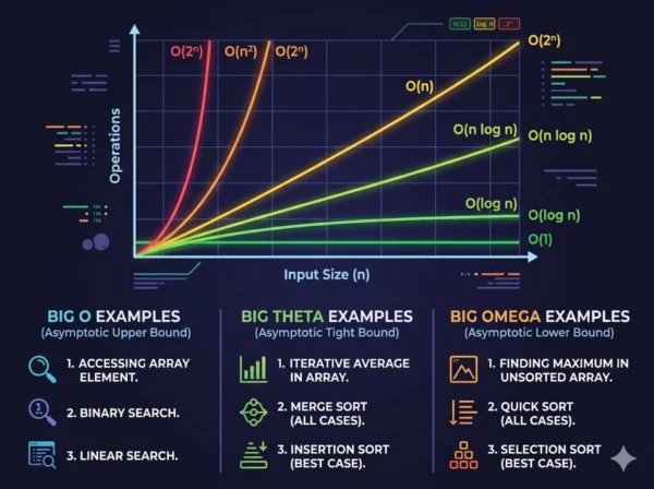
10 Critical Differences: Big O vs Big Theta vs Big Omega
Aspect | Big O Notation (O) | Big Theta Notation (Θ) | Big Omega Notation (Ω) |
|---|---|---|---|
| Bound Type | Upper bound — function grows no faster than f(n) | Tight bound — function grows at exactly the rate of f(n) | Lower bound — function grows no slower than f(n) |
| Mathematical Condition | T(n) ≤ c·f(n) for all n ≥ n₀ | c₁·f(n) ≤ T(n) ≤ c₂·f(n) for all n ≥ n₀ | T(n) ≥ c·f(n) for all n ≥ n₀ |
| Primary Question Answered | “How bad can this algorithm get?” | “What is the exact growth rate?” | “How fast must this algorithm always be?” |
| Bound Strictness | Can be loose; O(n²) is valid even for O(n) functions | Must be tight; no slack between upper and lower constants | Can be loose; Ω(1) is valid for any function |
| Typical Use Context | Worst-case analysis, capacity planning, interview communication | Precise academic analysis, proving algorithm optimality | Best-case analysis, problem complexity lower bound proofs |
| Industry Usage Frequency | Extremely common; standard notation in code reviews and design docs | Rare in practice; primarily appears in academic papers and textbooks | Rare in practice; primarily used in theoretical CS research |
| Relationship to Worst Case | Directly describes worst-case behavior when applied to worst-case input | Applies only when best and worst case have identical growth rates | Typically applied to best-case input analysis |
| Quicksort Example | O(n²) — worst case with already-sorted input and bad pivot | Θ(n log n) — average case over random inputs | Ω(n log n) — best case with good pivot selection |
| Optimality Expression | Cannot express optimality; only provides a ceiling | Expresses optimality when Theta matches proven problem lower bound | Establishes that an algorithm cannot be improved beyond this floor |
| Notation Symbol Origin | O from German “Ordnung” (order) via Bachmann-Landau notation | Θ (theta) introduced by Knuth in 1976 for tight asymptotic bounds | Ω (omega) introduced by Knuth in 1976 as complement to Big O |
Practical Implementation and Code Examples
Step-by-Step Complexity Analysis
- Identify the input variable: First, establish what n represents — array length, node count, character count, or another quantity that grows with problem size.
- Identify dominant operations: Then, locate the operations that execute most frequently — comparisons in a sort, additions in matrix multiply, lookups in a search.
- Count operation frequency: Additionally, express how many times each dominant operation executes as a function of n, tracking loop iterations and recursive calls.
- Identify best and worst case inputs: Furthermore, determine which input arrangement triggers maximum operations (worst case) and minimum operations (best case).
- Express each case with appropriate notation: Subsequently, use Big O for worst case, Omega for best case, and Theta only when both bounds are identical.
- Drop constants and low-order terms: Finally, simplify by keeping only the dominant term and dropping coefficients: 3n² + 5n + 7 becomes O(n²).
Code Examples with Full Notation Analysis
O(1) — Constant Time
// Array index access — always one operation
int getElement(int[] arr, int index) {
    return arr[index]; // O(1)
}

// Hash map lookup — amortized constant
String getValue(HashMap<String, String> map,
                String key) {
    return map.get(key); // O(1) average, O(n) worst
}
Big O: O(1) | Big Theta: Θ(1) for array access | Big Omega: Ω(1)
Array index access has identical complexity for all inputs — a perfect tight bound exists.
O(n) — Linear Time
// Linear search
int linearSearch(int[] arr, int target) {
    for (int i = 0; i < arr.length; i++) {
        if (arr[i] == target) return i; // O(1) if first
    }
    return -1; // O(n) if not found
}

// Sum all elements
int sumArray(int[] arr) {
    int sum = 0;
    for (int num : arr) sum += num; // always n ops
    return sum; // Θ(n) tight bound
}
Linear Search: O(n) worst, Ω(1) best (first element), no tight bound.
Sum Array: Θ(n) tight — always visits every element regardless of input.
O(log n) — Logarithmic Time
// Binary search on sorted array
int binarySearch(int[] arr, int target) {
    int left = 0, right = arr.length - 1;
    while (left <= right) {
        int mid = left + (right - left) / 2;
        if (arr[mid] == target) return mid; // Ω(1) best
        if (arr[mid] < target) left = mid + 1;
        else right = mid - 1;
    }
    return -1; // O(log n) worst case
}
Big O: O(log n) | Big Theta: Θ(log n) worst case | Big Omega: Ω(1) if middle element matches. Halves search space each iteration.
O(n²) — Quadratic Time
// Bubble sort
void bubbleSort(int[] arr) {
    int n = arr.length;
    for (int i = 0; i < n - 1; i++) {         // n
        for (int j = 0; j < n - i - 1; j++) { // n
            if (arr[j] > arr[j + 1]) {
                int temp = arr[j];
                arr[j] = arr[j + 1];
                arr[j + 1] = temp;
            }
        }
    }
} // O(n²) worst and average case
Big O: O(n²) | Big Theta: Θ(n²) for standard implementation | Big Omega: Ω(n) with early-exit optimization on sorted input.
Best Practices for Complexity Analysis
Good Analysis Habits
- Always specify which case you are analyzing: worst, average, or best
- Use Theta only when you can prove both bounds with identical growth functions
- Analyze space complexity alongside time complexity for complete characterization
- Consider amortized complexity for data structures with occasional expensive operations
- Verify complexity claims empirically with timing benchmarks on realistic input sizes
- Account for cache behavior — O(n) with poor locality can outperform O(n log n) with excellent locality for practical n
Common Mistakes to Avoid
- Never conflate Big O with worst case — they are independent concepts that happen to align frequently
- Avoid claiming Theta without proving both the upper and lower bounds rigorously
- Don’t ignore constant factors for small n where they dominate the actual runtime
- Resist the temptation to use Omega for best-case optimization decisions in production systems
- Never dismiss an algorithm as slow based on Big O alone without considering typical input distributions
- Avoid comparing algorithms across wildly different constant factors using Big O notation alone
Complexity Classes and Real-World Performance
Acceptable Complexity
O(1), O(log n), O(n): Scale to billions of inputs
O(n log n): Practical for tens of millions of inputs
Target: Production systems should aim here
Caution Zone
O(n²): Acceptable for n under ~10,000
O(n³): Practical only for n under ~1,000
Context: Justify before deploying at scale
Intractable Territory
O(2ⁿ), O(n!): Only feasible for very small n
NP-hard problems: Use heuristics or approximations
Note: Avoid in any scalable system design
Operations Per Second Reality Check
| Complexity | n = 10 | n = 1,000 | n = 1,000,000 | At 10⁹ ops/sec: n=1M takes |
|---|---|---|---|---|
| O(1) | 1 | 1 | 1 | < 1 nanosecond |
| O(log n) | 3 | 10 | 20 | < 1 nanosecond |
| O(n) | 10 | 1,000 | 1,000,000 | ~1 millisecond |
| O(n log n) | 33 | 10,000 | 20,000,000 | ~20 milliseconds |
| O(n²) | 100 | 1,000,000 | 10¹² | ~17 minutes |
| O(2ⁿ) | 1,024 | 10³⁰¹ (astronomical) | Infinite (effectively) | Heat death of universe |
The Constant Factor Reality:
Asymptotic notation deliberately drops constant factors, but those factors matter profoundly in practice. A carefully optimized O(n²) algorithm with SIMD vectorization may outperform a naive O(n log n) algorithm for all practical input sizes your system encounters. Similarly, an O(log n) algorithm with poor cache behavior can run slower than an O(n) algorithm that processes memory sequentially. Use asymptotic notation to eliminate clearly inferior choices, then benchmark real implementations on realistic inputs before committing to a final design. Just as infrastructure decisions require benchmarking real workloads rather than relying purely on theoretical comparisons, algorithm selection ultimately demands empirical validation alongside theoretical analysis.
When to Use Each Notation
Choosing the Right Notation for Your Context
The three notations are not competing alternatives — they answer different questions. The right choice depends entirely on what you are trying to communicate and to whom. In a technical interview, Big O is almost always the expected answer. In an academic proof of algorithm optimality, Theta and Omega become essential. In a research paper establishing that a problem cannot be solved faster than a certain rate, Omega is the central tool. Understanding which question you are answering determines which notation you should reach for.
Decision Matrix
| Situation | Use Big O When… | Use Big Theta When… | Use Big Omega When… |
|---|---|---|---|
| Technical Interview | Almost always — it is the expected standard answer | When asked for tight bounds or to prove optimality | When asked specifically about best case |
| Code Documentation | Standard choice for documenting function complexity | When function has identical best and worst case performance | Rarely used in code-level documentation |
| System Design | Capacity planning and worst-case load estimation | When precise bound is known and tightness matters for design | Bounding minimum resource requirements |
| Academic Paper | Bounding algorithm complexity from above | Proving exact asymptotic complexity of algorithms | Proving lower bounds for problems or algorithm classes |
| Algorithm Comparison | Initial screening to eliminate clearly inferior options | Comparing algorithms with identical tight bounds | Establishing whether one algorithm is provably better than another |
| Optimization Work | Identifying the complexity class to target for improvement | Confirming an optimized algorithm matches the theoretical bound | Determining whether further optimization is theoretically possible |
Practical Notation Application Patterns
Industry Engineering Context
Academic and Research Context
Strategic Recommendation for Students and Practitioners:
Master Big O first and thoroughly — it covers 90% of practical use cases. Then develop intuition for when a function has a tight bound (Theta) by practicing with algorithms like merge sort, heap sort, and matrix multiplication where best and worst cases are identical. Finally, study Big Omega in the context of sorting lower bound proofs and NP-completeness, where it appears most powerfully. Similar to how choosing the right automation approach requires understanding the problem’s inherent complexity constraints, choosing the right algorithmic approach requires knowing not just the upper bound but also the theoretical minimum work any algorithm must perform for the problem at hand.
Frequently Asked Questions: Big O, Big Theta, and Big Omega
Mastering Asymptotic Notation in 2026
The distinctions between Big O, Big Theta, and Big Omega notation form the bedrock of rigorous algorithm analysis. Big O gives you the safety guarantee you need for production systems — a ceiling that holds under the worst conditions your users can generate. Big Theta gives you the precision you need for academic proofs and optimal algorithm design — an exact characterization that eliminates all ambiguity. Big Omega gives you the floor you need for theoretical completeness — a lower bound that establishes what is impossible, not merely what is difficult.
Big O — Your Daily Tool
- Upper bound on growth rate
- Worst-case analysis standard
- Interview and documentation default
- Capacity planning foundation
- T(n) ≤ c·f(n) for large n
Big Theta — Precision Tool
- Tight bound — both upper and lower
- Exact growth rate characterization
- Academic and theoretical standard
- Optimality expression
- c₁·f(n) ≤ T(n) ≤ c₂·f(n) for large n
Big Omega — Theoretical Tool
- Lower bound on growth rate
- Best-case and optimality floor
- Problem hardness proofs
- Theoretical completeness
- T(n) ≥ c·f(n) for large n
Whether you are preparing for a software engineering interview, optimizing a production system under performance pressure, or studying computer science fundamentals, these three notations give you the complete vocabulary for algorithmic reasoning. Begin with Big O until it becomes instinctive, develop Theta fluency for any algorithm where tight bounds naturally exist, and reach for Omega when you need to establish what no algorithm can ever achieve. The result is not just better code — it is the ability to make claims about algorithms with mathematical rigor that separates engineering intuition from engineering precision.
Related Topics Worth Exploring
Master Theorem for Recurrences
Learn how to solve divide-and-conquer recurrence relations in O(1) analytical steps, covering all three cases and their Big O implications for recursive algorithm analysis.
P vs NP and Computational Complexity
Explore the unsolved question at the heart of computer science, how Big Omega lower bounds connect to NP-hardness proofs, and what polynomial versus exponential complexity means for algorithm design.
Data Structure Time Complexity Comparison
Compare arrays, linked lists, hash tables, balanced BSTs, and heaps across insertion, deletion, and search operations using all three asymptotic notations for complete performance analysis.