Merge sort splits, sorts and merges, always in O(n log n), and it needs extra memory. Quick sort partitions around a pivot and sorts in place, averaging O(n log n) with an O(n squared) worst case. The textbook conclusion is that merge sort is the safer pick. Real standard libraries disagree, though, and they disagree in an instructive way. Java sorts primitives with a Dual-Pivot Quicksort and objects with a merge-based TimSort. The deciding factor there is stability, not the worst case, because that worst case is engineered away in practice.
Both algorithms are divide and conquer, both average O(n log n), and both appear in every syllabus. Choosing between them is where most explanations stop being useful.
This guide checks what production libraries actually do. The Java API documentation and the C++ working draft both state their choices plainly. Those choices are not the ones the textbook comparison predicts.
How Each One Works
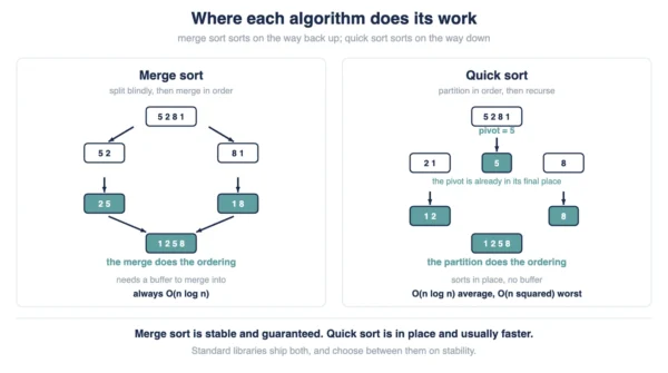
Merge sort divides first and does its work on the way back up. It splits the array in half, sorts each half recursively, then merges the two sorted halves into one. The merge step is where the ordering actually happens.
Quick sort, by contrast, inverts that. It picks a pivot, then partitions so smaller elements sit left and larger ones sit right. After that it recurses on each side. Here the partition step does the work, and no merge is needed.
That structural difference explains almost everything else. Merge sort’s split is always even, so its recursion depth is predictable. Quick sort’s split, however, depends entirely on the pivot it happens to choose.
Time Complexity, Worst Case Included
Merge sort runs in O(n log n) in the best, average and worst case. The halving never depends on the data, so nothing in the input can degrade it. Our Big O vs Big Theta vs Big Omega guide covers why those three cases are stated separately.
Quick sort averages O(n log n) too. Its worst case is O(n squared), though, and that happens when partitioning is maximally unbalanced. A pivot that is always the smallest or largest remaining element produces exactly that.
The classic trigger is an already-sorted array with a naive first-element pivot. Each partition then peels off one element, so the recursion depth becomes n rather than log n. Our time complexity guide covers how that depth drives the total.
What Each One Costs in Memory
Quick sort partitions in place. Beyond the recursion stack it needs only a constant amount of extra space. Our stack vs heap guide puts that stack in context.
Merge sort, by contrast, needs somewhere to merge into. A standard array implementation allocates O(n) auxiliary space, and that allocation is the price of the guaranteed bound.
Java’s object sort is more nuanced than the textbook figure suggests. Its temporary storage requirements “vary from a small constant for nearly sorted input arrays”, per the API documentation. Randomly ordered input instead costs “n/2 object references”.
Note what that means. The O(n) figure is a worst case for merge sort, not a fixed cost. So a good implementation pays far less on partially ordered data.
Merge Sort vs Quick Sort: Comparison Table
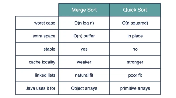
The table below lines up the two algorithms, field by field. Every entry reflects the standard array implementations.
| Aspect | Merge Sort | Quick Sort |
|---|---|---|
| Strategy | Divide evenly, then merge | Partition around a pivot, then recurse |
| Where the work happens | In the merge, on the way back up | In the partition, on the way down |
| Best case | O(n log n) | O(n log n) |
| Average case | O(n log n) | O(n log n) |
| Worst case | O(n log n) | O(n squared) |
| What triggers the worst case | Nothing in the input | Repeatedly unbalanced partitions |
| Extra space | O(n) auxiliary | In place, plus the recursion stack |
| Stable | Yes | No, not in the usual in-place form |
| Cache behaviour | Weaker; merging touches two regions | Stronger; partitioning is local |
| Suits linked lists | Yes, no random access needed | Poorly, partitioning wants indexing |
| Suits arrays | Yes, at the cost of the buffer | Yes, and usually faster in practice |
| Parallelises | Readily; halves are independent | Readily; partitions are independent |
| External sorting | The standard choice | Rarely used |
| Java uses it for | Object arrays, as TimSort | Primitive arrays, dual-pivot |
| C++ equivalent | std::stable_sort | std::sort, usually via introsort |
| Deciding factor in practice | Stability is required | Speed and memory matter more |
The last three rows carry the real answer. Both algorithms ship in the same standard libraries, chosen for different jobs.
Stability, the Deciding Difference
A stable sort preserves the relative order of equal elements. Sort employees by department after sorting by name, and a stable sort keeps each department’s names alphabetical. An unstable sort, however, may scramble them.
Merge sort, then, is naturally stable. When the merge step meets two equal elements, taking the left one first preserves the original order at no cost.
Quick sort is not stable in its usual in-place form. Partitioning swaps distant elements, which destroys the original relative order of equal keys. Making it stable requires extra space, which removes its main advantage.
Java’s documentation states the guarantee directly for object sorting. That sort “is guaranteed to be stable: equal elements will not be reordered as a result of the sort”.
What Standard Libraries Actually Choose
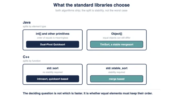
Here is the fact that settles the which is better question. Java uses both, in the same class, and splits them by element type.
For primitive arrays the documentation is explicit. The algorithm “is a Dual-Pivot Quicksort by Vladimir Yaroslavskiy, Jon Bentley, and Joshua Bloch”. It “offers O(n log(n)) performance on all data sets”. It is also “typically faster than traditional (one-pivot) Quicksort implementations”.
For object arrays, though, it switches. That implementation is “a stable, adaptive, iterative mergesort”, and it “was adapted from Tim Peters’s list sort for Python (TimSort)”.
The reason is stability rather than speed. Two equal integers are interchangeable, so stability is meaningless for primitives. Two objects that compare equal may differ in every other field, so their order matters.
C++ splits the same way, by function rather than by type. The standard requires “O(NlogN) comparisons and projections” for std::sort and says nothing about stability. std::stable_sort is stable. It costs “Nlog(N) comparisons” only when enough extra memory is available, and “at most Nlog2(N) comparisons” otherwise.
Why the Worst Case Rarely Bites
The O(n squared) worst case is real, and it is also the most over-weighted fact in this comparison. Production implementations do not ship plain quick sort.
C++ makes that a requirement rather than a preference. The standard demands “O(NlogN) comparisons and projections” from std::sort, so a naive quicksort would not conform at all.
Implementations meet that bound with introsort, which Musser introduced in 1997. It starts as quicksort, switches to heapsort once recursion depth passes a threshold, and finishes small ranges with insertion sort.
The result keeps quicksort’s speed and caps the damage. Java takes a different route to the same place. Its dual-pivot implementation reports “O(n log(n)) performance on all data sets”.
So the honest framing is narrower than the textbook one. Plain quick sort has an O(n squared) worst case, and the quick sort you actually call almost certainly does not.
Linked Lists Change the Answer
Everything above assumed arrays. On a linked list the comparison inverts, and the reason is random access.
Quick sort’s partition step wants to index into the middle of the range. A linked list makes that O(n) per access, as our array vs linked list guide explains.
Merge sort needs no indexing at all. It walks the list to split it, then merges by following pointers. So it works naturally on a structure with no random access.
Merge sort also drops its memory penalty here. Merging linked nodes only relinks pointers, so no auxiliary array is required. That is why linked-list sorts are almost always merge sorts.
Which One to Use
Reach for quick sort on arrays when you have no stability requirement. It sorts in place, its partitioning is cache-friendly, and the library version has already handled the worst case for you.
Reach for merge sort when equal elements must keep their order, or when you are sorting a linked list. Choose it too when you need a hard guarantee rather than an average, such as in latency-sensitive code.
Merge sort also owns external sorting. Data too large for memory gets sorted in chunks and merged in passes, which quick sort’s random access makes impractical.
Sorting often sits inside a larger algorithm too. Kruskal’s algorithm begins by sorting every edge by weight, a step our Prim’s vs Kruskal’s guide covers. There the sort is a subroutine, so the library choice is the whole decision.
In most application code the honest answer is to call the library. Java and C++ have both already made this decision, and they made it more carefully than a hand-rolled implementation will.
Interview Questions
Frequently Asked Questions
Wrapping Up
The textbook comparison ends at the worst case, and that is the least useful place to stop. Merge sort guarantees O(n log n) and is stable. Quick sort sorts in place and runs faster on arrays. Its worst case is also handled by every library you would realistically use.
Remember how the standard libraries decided. Java picks quicksort for primitives and mergesort for objects, and the axis it splits on is stability. That is the question worth asking of your own data.
Related reading on DiffStudy:
- Big O vs Big Theta vs Big Omega
- Understanding Time Complexity
- Array vs Linked List
- Stack vs Heap Memory Allocation
- Prim’s vs Kruskal’s Algorithm