Both Prim’s and Kruskal’s are greedy algorithms that find the Minimum Spanning Tree of a weighted graph. Prim’s grows one tree from a start vertex, always adding the cheapest edge to a new vertex. Kruskal’s sorts all edges and adds the cheapest one that does not form a cycle. So Prim’s is vertex-based and Kruskal’s is edge-based, and both give an MST of the same total weight.
Prim’s and Kruskal’s are the two classic algorithms for building a Minimum Spanning Tree. They are a staple of DSA courses and GATE exams, and students often mix up how each one picks its edges.
Both reach the same goal by a greedy path, but they get there differently. This guide defines a spanning tree, explains each algorithm with examples, compares them in detail, and shows when to use which.
They build on graph basics, so it helps to know the difference between a graph and a tree first.
What is a Minimum Spanning Tree?
A spanning tree of a connected, weighted graph connects all the vertices with the fewest edges and no cycles. For a graph with V vertices, a spanning tree always has exactly V minus 1 edges. A graph can have many spanning trees.
The Minimum Spanning Tree (MST) is the spanning tree with the lowest total edge weight. Both Prim’s and Kruskal’s algorithms find this MST. They are used in network design, such as laying cable, pipelines, or roads at the least total cost.
What is Prim’s Algorithm?
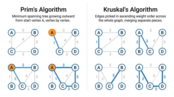
Prim’s algorithm is a greedy, vertex-based method. It starts at any one vertex and grows a single tree outward. At each step it adds the cheapest edge that connects a vertex already in the tree to a vertex outside it.
It keeps going until every vertex is included. To find the cheapest connecting edge quickly, it uses a priority queue or min-heap. By construction, it never creates a cycle.
Advantages of Prim’s:
- Efficient on dense graphs, where edges are plentiful.
- Simple to implement with a priority queue or an adjacency matrix.
- Builds one connected tree throughout, which is easy to reason about.
Disadvantages of Prim’s:
- Less efficient on sparse graphs than Kruskal’s.
- Needs a connected graph to span every vertex.
- Harder to parallelise because the tree grows in sequence.
Complexity: time is O(E log V) with a binary heap, or O(V²) with an adjacency matrix. Space is O(V) for the priority queue and vertex tracking.
What is Kruskal’s Algorithm?
Kruskal’s algorithm is a greedy, edge-based method. It first sorts all the edges by weight. Then it adds the next cheapest edge, as long as that edge does not form a cycle.
It starts with every vertex as its own piece and merges them into one tree. To check whether an edge would form a cycle, it uses a Union-Find (disjoint set) structure.
Advantages of Kruskal’s:
- Efficient on sparse graphs, where edges are few.
- Works on a disconnected graph too, returning a minimum spanning forest.
- Easier to parallelise, since independent edges can be considered together.
Disadvantages of Kruskal’s:
- Slower on dense graphs because sorting many edges is costly.
- Needs a Union-Find structure, which adds implementation effort.
- Sorting the full edge list dominates the running time.
Complexity: time is O(E log E), which is the same as O(E log V), dominated by sorting. Space is O(V + E) for the edge list and the disjoint set.
Prim’s vs Kruskal’s Algorithm: Comparison Table

| Aspect | Prim’s Algorithm | Kruskal’s Algorithm |
|---|---|---|
| Approach | Vertex-based (grows from a vertex) | Edge-based (sorts all edges) |
| Builds | One growing tree | A forest that merges into a tree |
| Edge selection | Cheapest edge to a new vertex | Globally cheapest edge with no cycle |
| Data structure | Priority queue / min-heap | Sorting + Union-Find (DSU) |
| Cycle handling | Never forms a cycle by design | Explicit cycle check (Union-Find) |
| Starting point | A chosen start vertex | No start; global edges |
| Time complexity | O(E log V) heap, O(V²) matrix | O(E log E) = O(E log V) |
| Space complexity | O(V) | O(V + E) |
| Best for | Dense graphs | Sparse graphs |
| Disconnected graphs | Needs a connected graph | Works (gives a spanning forest) |
| Negative weights | Handled fine | Handled fine |
| Parallelisation | Hard (sequential growth) | Easier (independent edges) |
| Memory use | More (queue + vertex tracking) | Less (mainly the disjoint set) |
| Strategy | Greedy | Greedy |
| Result | An MST | An MST of the same total weight |
Worked Example
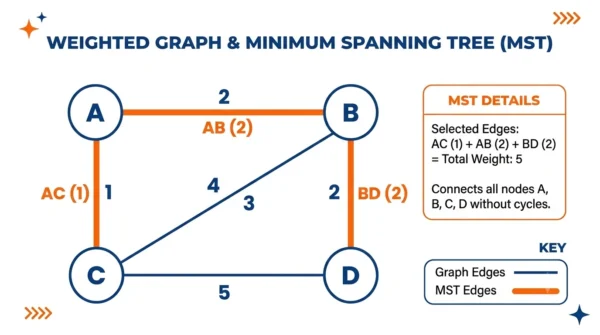
Take a graph with four vertices, A, B, C, and D, and these weighted edges: AB(2), AC(1), AD(4), BC(3), BD(2), CD(5). Both algorithms find the same minimum spanning tree.
Prim’s, starting at A:
- From A, the cheapest edge is AC(1). Add C.
- From the tree {A, C}, the cheapest new edge is AB(2). Add B.
- From {A, B, C}, the cheapest new edge is BD(2). Add D.
Kruskal’s, sorting edges:
- Sorted order: AC(1), AB(2), BD(2), BC(3), AD(4), CD(5).
- Add AC(1), then AB(2), then BD(2). Each joins two separate pieces, so none forms a cycle.
Both produce the MST {AC, AB, BD} with a total weight of 5. The tree has 3 edges for 4 vertices, as expected.
How They Work, Step by Step
Prim’s follows these steps:
- Pick any start vertex and add it to the tree.
- Find the cheapest edge from the tree to a vertex not yet in it.
- Add that edge and vertex, then repeat until all vertices are included.
Kruskal’s follows these steps:
- Sort every edge by weight, from smallest to largest.
- Take the next cheapest edge and add it if it joins two separate pieces.
- Skip any edge that would form a cycle, and repeat until the tree is complete.
Applications of MST Algorithms
Minimum spanning trees solve real “least total cost to connect everything” problems, so both algorithms show up widely.
- Network and circuit design: laying cables, pipelines, roads, or wiring a circuit board at the lowest total cost.
- Cluster analysis: grouping similar data points, where Kruskal’s edge order is handy.
- Image segmentation: splitting an image into regions based on pixel similarity.
- Approximation algorithms: building blocks for problems like the travelling salesman.
Prim’s is common in dense network problems, while Kruskal’s suits sparse graphs and clustering.
When to Use Prim’s or Kruskal’s
Use Prim’s when the graph is dense, with many edges. Growing from a vertex with a priority queue is efficient there, and it avoids sorting a huge edge list.
Use Kruskal’s when the graph is sparse, with few edges. Sorting a short edge list is cheap, and Union-Find makes the cycle checks fast. Kruskal’s also handles a disconnected graph by returning a spanning forest.
Either way, both return a minimum spanning tree of the same total weight, so the choice is about graph shape, not the result.
Interview Questions
Frequently Asked Questions
Wrapping Up
Prim’s and Kruskal’s both build a minimum spanning tree, but from different angles. Prim’s grows one tree from a vertex with a priority queue, while Kruskal’s sorts edges and joins pieces with Union-Find.
Remember the simple rule: Prim’s suits dense graphs and Kruskal’s suits sparse graphs. Both are greedy, both handle negative weights, and both return an MST of the same total cost.
Related reading on DiffStudy:
- Graph vs Tree
- DFS vs BFS
- Binary Tree vs Binary Search Tree
- Time Complexity of Data Structures
- CS Fundamentals hub