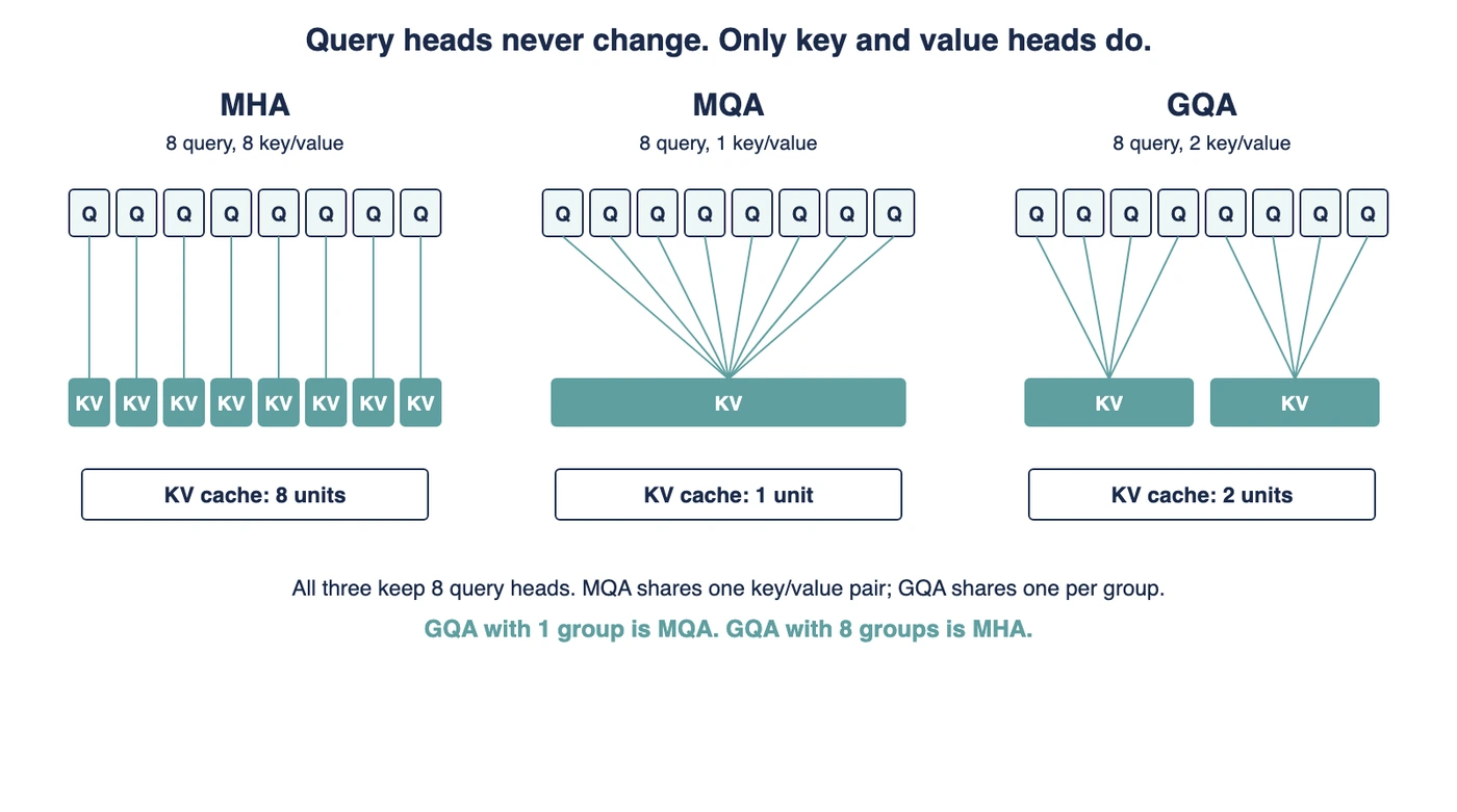
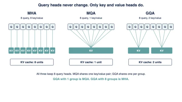
Multi-head attention gives every query head its own key head and value head. Multi-query attention keeps all those query heads, though one key head and one value head now serve every one of them. Grouped-query attention sits between the two, since each group of query heads shares a single key and value pair. Shazeer introduced multi-query attention in 2019. Ainslie and colleagues introduced grouped-query attention in 2023, calling it “an interpolation between multi-head and multi-query attention”. The query head count never moves. Only the key and value head count does.
A decoder produces one token per forward pass. At every pass it reloads the cached keys and values for each earlier position. That reload is the slow step, and it grows with sequence length.
Multi-query attention and grouped-query attention both shrink that cache. Neither one touches the query heads. Both cut how many key and value heads exist, so fewer bytes move per decoding step.
This guide reads the two source papers directly. Shazeer wrote the multi-query paper at Google in 2019. Ainslie and colleagues wrote the grouped-query paper at Google Research in 2023, and their measured tables settle most of the usual arguments.
Why Loading Keys and Values Is the Bottleneck
Attention heads turn up in encoder and decoder stacks alike, as our self-attention vs cross-attention guide sets out. Training runs those heads across the whole sequence at once. Incremental decoding cannot.
Shazeer frames the entire problem as “the ratio of memory access to arithmetic operations”. That ratio matters because accelerators are lopsided. He describes hardware “where the computational capacity can be two orders of magnitude higher than the memory bandwidth”.
During incremental decoding that ratio climbs toward one. Shazeer writes that this ends up “causing memory bandwidth to be a major performance bottleneck on modern computing hardware”. The chip then waits on memory rather than on arithmetic.
So what exactly gets reloaded? The cached keys and values from every earlier position, at every single step. Shazeer’s abstract names the memory-bandwidth cost of repeatedly loading those large tensors as the core problem.
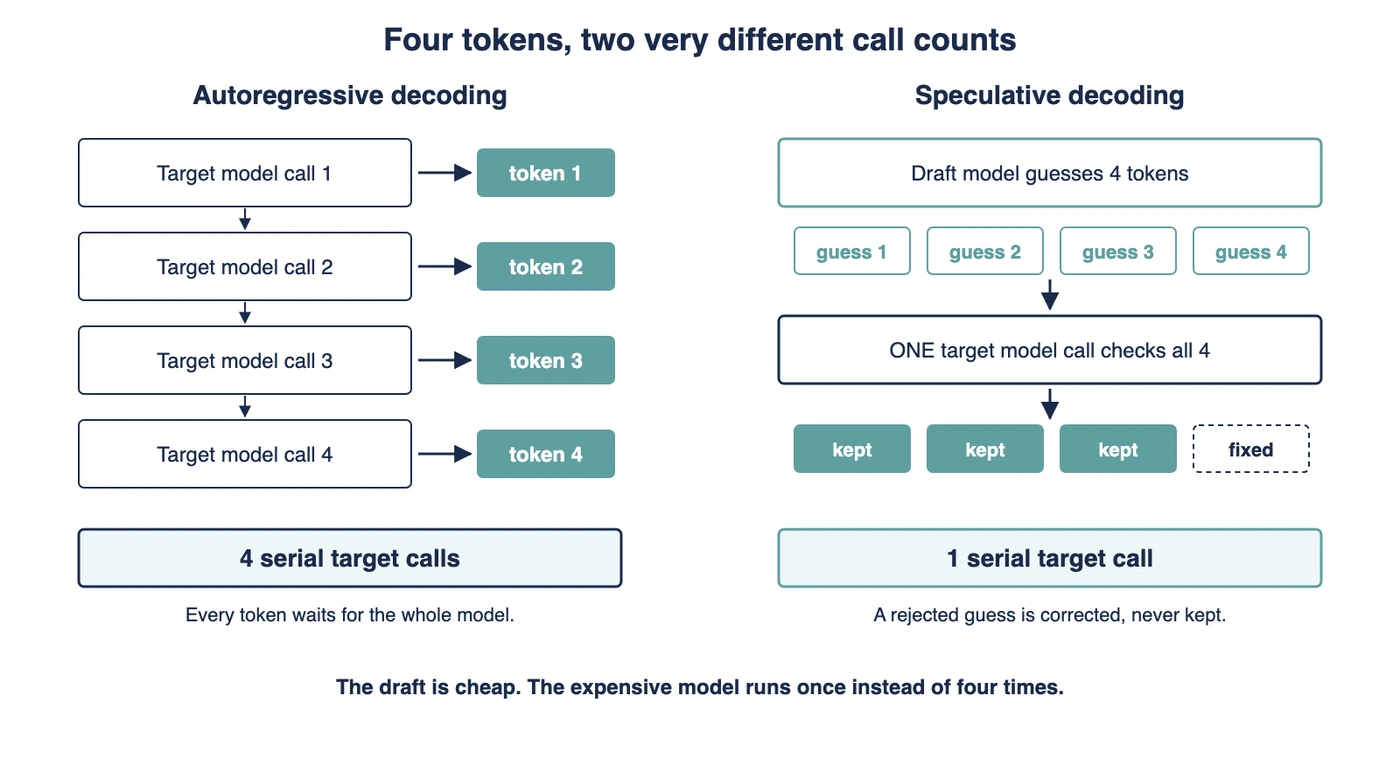
Serial decoding is also the target of speculative decoding, though from another angle. Speculative decoding cuts how many serial steps you run. Multi-query attention cuts the bytes each step must move. The two levers compose cleanly.
How Multi-Head Attention Works
Multi-head attention runs several attention layers side by side. Shazeer’s translation baseline uses eight heads, with key and value dimensions of 128. Every head owns a query projection, a key projection and a value projection.
Because each head owns its keys and values, the cache holds one set per head. That is the largest KV footprint among the three schemes. Nothing at all gets shared.
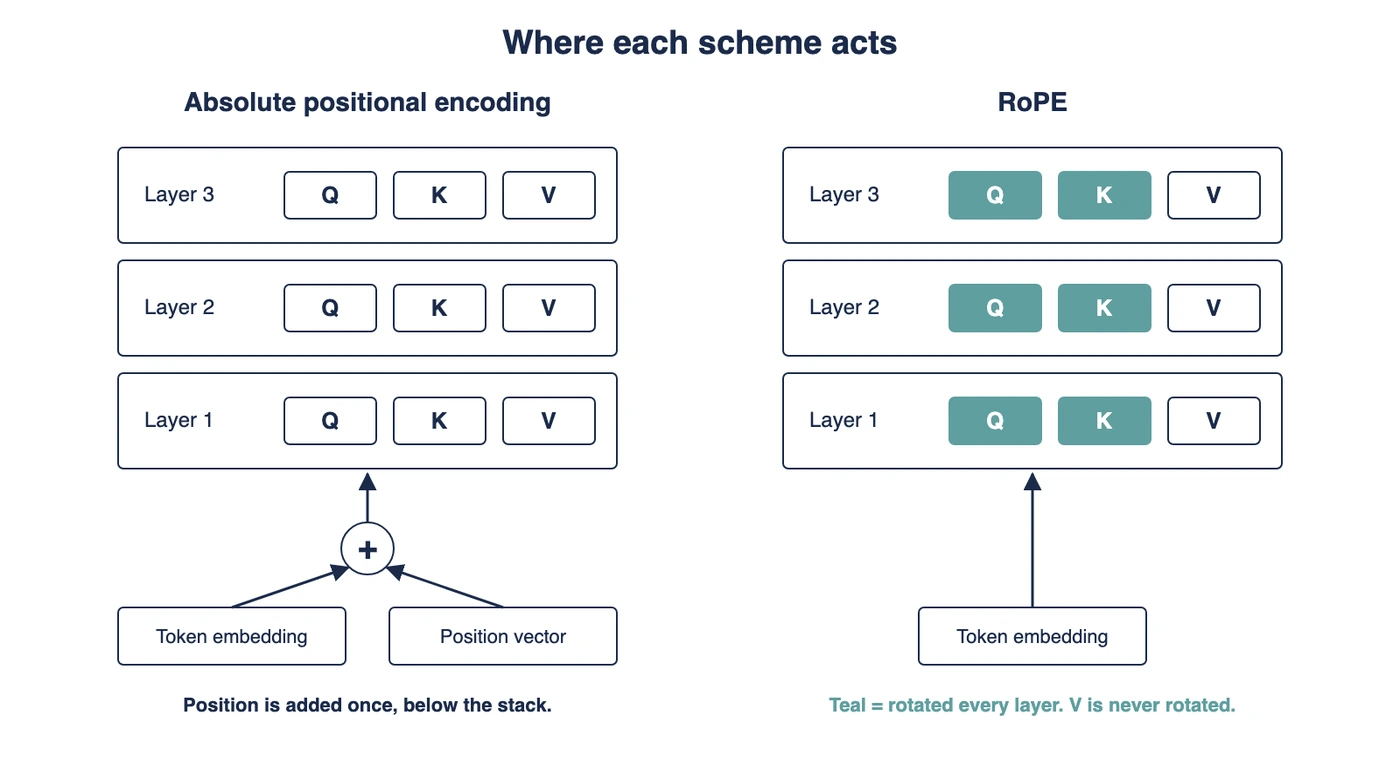
Queries and keys are also the tensors that positional schemes rewrite, as our RoPE vs absolute positional encoding guide covers. Head structure and position handling stay separate choices, though. Neither one forces the other.
Training this layer is quick, since the whole sequence runs in parallel. Decoding is where the bill arrives. Every step reloads eight sets of keys and values rather than one.
How Multi-Query Attention Works
Multi-query attention changes exactly one thing. The query heads stay untouched, while a single key head and a single value head serve all of them. Ainslie describes a scheme “which uses multiple query heads but single key and value heads”.
Their Figure 2 caption says it in one line. “Multi-query attention shares single key and value heads across all query heads.” Shazeer’s abstract makes the same point, since keys and values are shared across every attention head in his variant.
The KV cache therefore shrinks by the head count. With eight heads, a single set replaces eight sets. Fewer bytes then move at every decoding step.
Notice what did not change here. The number of query heads is identical to the multi-head baseline. Only the key and value head count moved, and that one detail is what most explanations blur.
How Grouped-Query Attention Works
Grouped-query attention is a dial rather than a third mechanism. Ainslie and colleagues define it as “an interpolation between multi-head and multi-query attention with single key and value heads per subgroup of query heads”.
Query heads split into G groups. Each group shares one key head and one value head. GQA-8 therefore names eight groups, so eight key and value pairs survive.
Both endpoints matter here. With one group, grouped-query attention is exactly multi-query attention. With as many groups as query heads, it is exactly multi-head attention. Everything between those endpoints is a tunable middle.
Why add the dial at all? Because “multi-query attention (MQA) can lead to quality degradation and training instability”, in the newer paper’s own words. A gentler cut keeps more of the baseline quality.
You also do not need a fresh training run. The recipe uptrains existing multi-head checkpoints “using 5% of original pre-training compute”. First “The key and value heads are mean-pooled to the appropriate MQA or GQA structure”. Then the model gets pre-trained a little longer.
MHA vs MQA vs GQA: Comparison Table
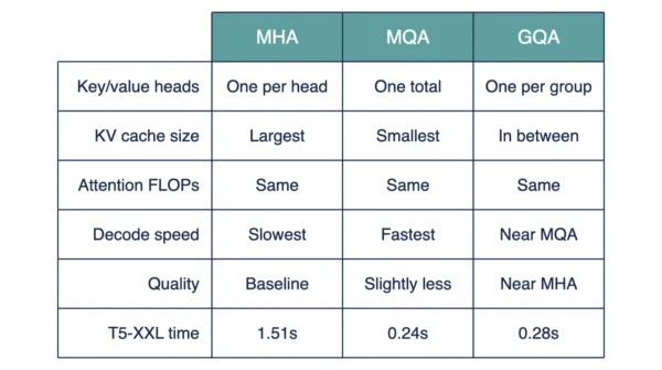
The table below sets the three schemes side by side, row by row. Every value traces back to one of the two papers named above.
| Aspect | MHA (multi-head) | MQA (multi-query) | GQA (grouped-query) |
|---|---|---|---|
| Query heads per layer | Eight, when following Shazeer’s baseline | Still eight, exactly as in MHA | Still eight, since query heads never change |
| Key and value heads per layer | One pair per query head, namely eight | One pair in total, rather than eight | One pair per group, so eight for GQA-8 |
| What gets shared | Nothing, since every head owns its own | Keys and values, across all query heads | Keys and values, though only inside a group |
| KV cache size per token | Largest, when compared across the three | Smallest, namely one set instead of eight | Between the two, since G sets survive |
| Attention arithmetic per token | The baseline amount, still the reference | Essentially unchanged, rather than reduced | Essentially unchanged as well |
| What the real bottleneck is | Memory bandwidth, when decoding serially | Memory bandwidth too, though far less of it | Memory bandwidth again, tuned by group count |
| Decoder inference speed | 46 microseconds per token, also 203 with beam-4 | 3.8 microseconds, while beam-4 drops to 32 | Not in Shazeer’s table, since GQA came later |
| Training speed | 13.2 microseconds, generally untouched | 13.0 microseconds, so barely different | Not reported in the 2019 tables either |
| Quality against the MHA baseline | The baseline itself, namely the reference row | “slightly worse than the baseline”, per Shazeer | “quality close to multi-head attention”, when uptrained |
| Training stability | Stable, still the reference case | Ainslie report “quality degradation and training instability” | Introduced partly because of that instability |
| A special case of another scheme | Yes, since GQA with eight groups is MHA | Yes, since GQA with one group is MQA | No, rather it is the general form of both |
| How to get one from an MHA checkpoint | Already the starting point, so nothing to do | Mean-pool the key and value heads, then uptrain | Mean-pool into groups, then uptrain likewise |
| Paper and year | The baseline in both papers, 2019 and 2023 | Shazeer, arXiv 1911.02150, 2019 | Ainslie and colleagues, arXiv 2305.13245, 2023 |
| Measured T5 inference time | 0.37s at Large, though 1.51s at XXL | 0.24s at XXL, still the fastest row | 0.28s at XXL, so very close to MQA |
| Measured T5 average score | 46.0 at Large, while XXL reaches 47.2 | 46.6 at XXL, above MHA-Large | 47.1 at XXL, nearly matching MHA-XXL |
| Dev ln(PPL) on WMT14 EN-DE | 1.424, namely the baseline row | 1.439, so slightly worse than MHA | Not measured, since the paper came later |
| Where it turns up today | Named by Ainslie as common, including T5 and LLaMA | Named by Ainslie as already used in PaLM | Proposed when MHA quality and MQA speed both matter |
One row above deserves a second look, namely attention arithmetic per token. All three schemes compute roughly the same amount. The next section shows why that matters so much.
The Arithmetic Barely Changes
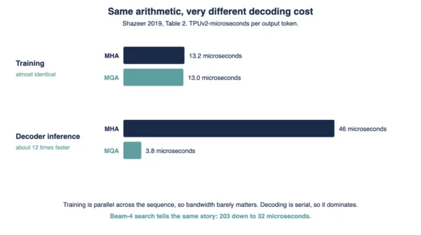
People often describe multi-query attention as a way to make attention cheaper to compute. That description gets the trade backward. The attention computation per token is essentially unchanged.
What actually falls is the number of key and value bytes reloaded at each decoding step. This is a KV-cache story, not a FLOPs story. Shazeer’s framing is “the ratio of memory access to arithmetic operations”, never the arithmetic alone.
His Table 2 proves the point better than any argument could. It reports TPUv2-microseconds per output token, at sequence length 128.
| Attention type | Training | Inference, enc + dec | Beam-4 search, enc + dec |
|---|---|---|---|
| multi-head | 13.2 | 1.7 + 46 | 2.0 + 203 |
| multi-query | 13.0 | 1.5 + 3.8 | 1.6 + 32 |
| multi-head local | 13.2 | 1.7 + 23 | 1.9 + 47 |
| multi-query local | 13.0 | 1.5 + 3.3 | 1.6 + 16 |
Read the two leftmost number columns together. Training moves from 13.2 to 13.0 microseconds, which is essentially nothing. Decoder inference moves from 46 to 3.8 microseconds, which is enormous.
Same model, same arithmetic, two completely different outcomes. Training runs in parallel across the sequence, so bandwidth barely constrains it. Decoding runs serially, so bandwidth dominates it.
Beam search tells the same story again. The decoder cost falls from 203 microseconds to 32. Encoder cost hardly budges, moving from 2.0 to 1.6, because the encoder was never the bandwidth problem.
What Multi-Query Attention Actually Costs
None of this comes free. Shazeer concedes that his models “incur only minor quality degradation from the baseline”. The 2023 paper is blunter, warning that “multi-query attention (MQA) can lead to quality degradation and training instability”.
Be fair to multi-query attention, though, because the lazy framing misses the real claim. Shazeer’s argument is comparative rather than absolute. If you want a smaller KV footprint, the obvious alternative is shrinking the heads themselves.
| Attention type | h | dk, dv | dff | ln(PPL) dev | BLEU dev | BLEU test, beam 1 / 4 |
|---|---|---|---|---|---|---|
| multi-head | 8 | 128 | 4096 | 1.424 | 26.7 | 27.7 / 28.4 |
| multi-query | 8 | 128 | 5440 | 1.439 | 26.5 | 27.5 / 28.5 |
| multi-head local | 8 | 128 | 4096 | 1.427 | 26.6 | 27.5 / 28.3 |
| multi-query local | 8 | 128 | 5440 | 1.437 | 26.5 | 27.6 / 28.2 |
| multi-head | 1 | 128 | 6784 | 1.518 | 25.8 | |
| multi-head | 2 | 64 | 6784 | 1.480 | 26.2 | 26.8 / 27.9 |
| multi-head | 4 | 32 | 6784 | 1.488 | 26.1 | |
| multi-head | 8 | 16 | 6784 | 1.513 | 25.8 |
The bottom four rows are the control group. Each one shrinks the head count or the head dimensions instead. Every single one scores worse than multi-query attention on dev perplexity.
That is the whole point of the table. Shazeer writes that “the multi-query attention model seems to be slightly worse than the baseline, but much closer than any of the alternatives involving decreasing h, dk and dv”. The language-model benchmark repeats the pattern, where multi-query reaches 30.2 dev perplexity against the multi-head baseline at 29.9. Every naive shrinking variant lands between 30.9 and 31.2.
Shazeer restates the finding plainly for that benchmark. “The multi-query attention model was slightly worse than the baseline, but significantly better than any of the alternatives involving decreasing h, dk and dv.”
Now for the number that gets misread most often. Shazeer notes that multi-query “actually had the highest BLEU score (28.5) with beam-4 decoding”. Read that against the rest of its own row, though. Dev ln(PPL) is worse, at 1.439 against 1.424. Dev BLEU is worse too, at 26.5 against 26.7.
So do not read 28.5 as multi-query beating multi-head. The paper’s own summary calls it “slightly worse than the baseline”. One test number landing 0.1 higher is noise, rather than a quality gain. Multi-query attention is not better than multi-head attention here.
What GQA Measured
Ainslie and colleagues measured T5 models with all three schemes. They uptrained T5-XXL checkpoints at proportion alpha = 0.05, which took approximately 600 TPUv3 chip-days. Their headline table reports inference time in seconds, alongside an average over all datasets.
| Model | Inference time (s) | Average |
|---|---|---|
| MHA-Large | 0.37 | 46.0 |
| MHA-XXL | 1.51 | 47.2 |
| MQA-XXL | 0.24 | 46.6 |
| GQA-8-XXL | 0.28 | 47.1 |
Look at MHA-Large against the two XXL variants below it. MQA-XXL runs at 0.24 seconds and scores 46.6. GQA-8-XXL runs at 0.28 seconds and scores 47.1. MHA-Large is slower, at 0.37 seconds, while scoring lower at 46.0.
That comparison is the strongest single result in either paper. A bigger model with fewer key and value heads beats a smaller model with full multi-head attention. It wins on speed and on quality at the same time.
Grouped-query attention then closes most of the remaining gap. GQA-8-XXL scores 47.1 against 47.2 for MHA-XXL, while running roughly five times quicker. The abstract summarises it well, since “uptrained GQA achieves quality close to multi-head attention with comparable speed to MQA”.
One more finding cuts against a common assumption. Bigger models do not suffer relatively more from the KV cache. Ainslie and colleagues note that “larger models suffer relatively less from memory bandwidth overhead from attention”, because the cache grows with model dimension while FLOPs and parameters grow with its square.
Which One You Meet in Practice
Plain multi-head attention remains the thing you meet in most textbooks and most older checkpoints. Ainslie name T5 and LLaMA as examples that did not use multi-query attention. Multi-head attention is also the baseline every comparison starts from.
Multi-query attention shows up where decode latency dominates everything else. Ainslie name PaLM as a model that already used it. The KV cache is smallest there, so long contexts and large batches both get cheaper.
Grouped-query attention is the setting you reach for when neither extreme fits. It gives you a knob rather than a choice between two fixed points. Pick more groups if quality slips; pick fewer if memory is tight.
Decoder-only inference is exactly where all this bites hardest, the family our BERT vs GPT guide contrasts with encoder stacks. Scaling the model up changes the calculus again, as our Mixture of Experts vs dense models guide explains. Sparse routing moves parameters off the critical path, while grouped-query attention moves cache bytes off it.
For an exam or an interview, lead with the head counts rather than the speedups. Say how many query heads each scheme keeps. Then say how many key and value heads it keeps. Those two numbers separate all three schemes immediately.
Interview Questions
Frequently Asked Questions
Wrapping Up
The three schemes differ along one axis only. Query heads stay constant, while the key and value head count drops from one per head, to one per group, to one in total.
Keep three measured facts past the acronyms. Training time barely moves, from 13.2 to 13.0 microseconds, though decoder inference falls from 46 to 3.8. Multi-query attention is slightly worse than the baseline, yet much better than naively shrinking heads. Grouped-query attention recovers most of that gap, since GQA-8-XXL scores 47.1 against 47.2 for MHA-XXL.
Related reading on DiffStudy:
- Self-Attention vs Cross-Attention
- Speculative Decoding vs Autoregressive Decoding
- RoPE vs Absolute Positional Encoding
- Mixture of Experts vs Dense Models
- BERT vs GPT