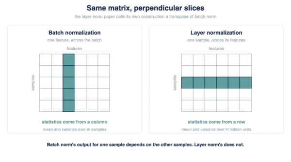
Batch normalization and layer normalization do the same job on a different axis. Batch norm averages down a column: one feature, across every sample in the mini-batch. Layer norm averages across a row instead: one sample, across its own features. The Layer Normalization paper describes this directly as a transpose of batch normalization. Because batch norm’s output depends on the other examples in the mini-batch, it needs stored running statistics, and it runs a different computation at inference. Layer norm depends on nothing but the sample itself, so it performs the same computation whether it is training or testing.
Every normalization layer averages activations before scaling them back. So the real question is simple. Which activations should share statistics first? Batch norm and layer norm answer that differently. So the gap runs through training stability, sequence models and inference alike. Readers new to either term can start with our machine learning and deep learning primer before continuing here.
This guide leans on two papers throughout. One is Sergey Ioffe and Christian Szegedy’s “Batch Normalization: Accelerating Deep Network Training by Reducing Internal Covariate Shift,” from Google. The other is Jimmy Ba, Jamie Kiros and Geoffrey Hinton’s “Layer Normalization,” from the University of Toronto. Both sit upstream of the choices inside blocks our self-attention vs cross-attention guide covers. So every formula and quote below traces back to one of them directly.
Why Normalize Activations at All
Ioffe and Szegedy named their target in the title: internal covariate shift. A layer’s inputs shift as earlier layers keep updating. So normalizing mid-network became the fix both papers pursue, each from a different axis.
Normalizing alone is not harmless, though. The BN paper is explicit that normalizing a layer’s inputs “may change what the layer can represent.” So the transform pairs with a learned scale and shift, on top of the normalized value. That pairing can still represent the identity. Neither paper treats it as optional.
How Batch Normalization Works
Batch normalization takes its statistics from a mini-batch of size m. Algorithm 1 in the BN paper lays out four steps for a value x_i.
mu_B      = (1/m) * sum of x_i
sigma_B^2 = (1/m) * sum of (x_i - mu_B)^2
x_hat_i   = (x_i - mu_B) / sqrt(sigma_B^2 + eps)
y_i       = gamma * x_hat_i + beta
mu_B is the mini-batch mean. sigma_B^2 is the mini-batch variance. x_hat_i is the normalized activation. y_i then applies the learned scale and shift, gamma and beta. Epsilon sits under the square root purely for stability. So the denominator never touches zero.
For a d-dimensional input, batch norm normalizes each dimension independently. So it never treats a layer as one block. Instead, it runs a separate mean and variance for every dimension, across the batch.
How Layer Normalization Works
Layer normalization takes its statistics from a single training case instead. Equation 3 in the LN paper defines the mean and the standard deviation. Both come from the H hidden units in a layer.
mu    = (1/H) * sum over i of a_i
sigma = sqrt( (1/H) * sum over i of (a_i - mu)^2 )
H is the number of hidden units in that layer, not the batch size. The LN paper puts the contrast directly. The paper puts it precisely. “All the hidden units in a layer share the same normalization terms mu and sigma.” Yet “different training cases have different normalization terms.” So every sample in a batch gets its own mu and sigma, apart from every other sample.
Like BN, layer normalization gives each neuron its own adaptive bias and gain. That gain applies after normalization but before the non-linearity.
Batch vs Layer Normalization: Comparison Table
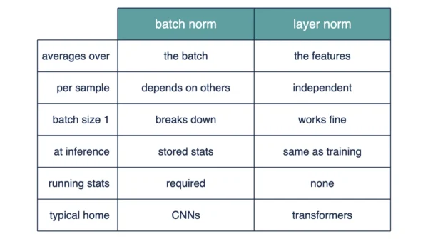
The table below lines up batch norm against layer norm, field by field. So every value traces back to one of the two papers directly.
| Aspect | Batch Normalization | Layer Normalization |
|---|---|---|
| Axis averaged over | Down a column: one feature, across the batch | Across a row instead: one sample, across its features |
| Statistics computed across | The mini-batch, per dimension | Instead, the H hidden units, per sample |
| Depends on other samples | Yes: output “depends both on the training example and the other examples in the mini-batch” | No, instead: output depends only on that one sample’s own features |
| Batch-size dependence | “Dependent on the mini-batch size,” per the LN paper | “Does not impose any constraint on the size of a mini-batch” |
| Behaviour at batch size 1 | Limited, since the same mini-batch-size dependence governs it | Explicitly supported: “the pure online regime with batch size 1” |
| Training vs inference | So it switches from mini-batch statistics to stored population statistics | “Performs exactly the same computation at training and test times” |
| Running statistics stored | Yes, so population mean and variance get tracked with moving averages | No, since statistics come fresh from each sample every time |
| Learned parameters | gamma and beta, one pair per dimension | An adaptive bias and gain, one pair per neuron |
| Where epsilon sits | Under the square root: sqrt(sigma_B^2 + eps) | Not part of the mean/variance formula as given in Eq. 3 |
| Suitability for RNNs | “Not obvious how to apply it to recurrent neural networks” | Instead, “straightforward to apply,” with statistics computed per time step |
| Variable-length sequences | Same dependence applies, since every time step forms a new batch | So computed per time step, independent of how long the sequence runs |
| Typical home | Feed-forward and convolutional networks, since that is the paper’s own target | Recurrent networks originally; transformer stacks later, since LN (2016) predates the Transformer (2017) |
| Year introduced | 2015 (Ioffe and Szegedy) | 2016 (Ba, Kiros and Hinton) |
| The paper’s own framing | The starting point, since LN’s own paper transposes it directly | “We transpose batch normalization into layer normalization” |
| What breaks as batches shrink | Statistics grow noisy, since the effect ties directly to mini-batch size | Nothing: its statistics never depended on batch size to begin with |
One row rewards a second look, the paper’s own framing. Layer norm is not a rival method invented from nothing. Instead, its own paper describes it as batch norm’s statistics, computed on a transposed axis. The next section unpacks that point fully.
The Transpose: Which Axis Gets Averaged
Picture one activation matrix. Samples run down the rows; features run across the columns. Batch norm and layer norm each average over one axis of that matrix. It is a different axis every time.
Batch norm averages down a column. That column is one feature, taken across every sample in the batch. Layer norm averages across a row instead. That row is one sample, taken across its own features.
The LN paper names this relationship directly. Ba, Kiros and Hinton describe their method as a transpose of batch normalization. The authors describe their own construction as a transpose. They “transpose batch normalization into layer normalization.” The statistics come “from all of the summed inputs to the neurons in a layer on a single training case.”
So the two methods are not two unrelated ideas. Instead, they are one operation, applied to perpendicular axes of the same matrix. Every difference the rest of this guide covers traces back to that single transpose.
Why One Sample’s Output Depends on the Others
Batch norm’s column average creates a side effect layer norm never has. Since the mean and variance come from the whole mini-batch, one sample’s output depends on its batch-mates.
The BN paper states this plainly. That dependence is stated outright. “The BN transform does not independently process the activation in each training example.” Rather, “BN(x) depends both on the training example and the other examples in the mini-batch.”
Layer norm carries no such dependency. Its mean and variance come from one sample’s own features. So nothing about another sample in the batch changes its output.
That single sentence from the BN paper is the root of every practical difference that follows. Batch norm needs running statistics because of it. So it behaves differently at inference too. Small batches hurt batch norm more than layer norm, as a result.
Why Batch Norm Changes at Inference
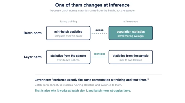
Depending on batch-mates suits training fine. It becomes a liability at test time, though. The BN paper explains the reason. That dependence “allows efficient training.” It is “neither necessary nor desirable during inference,” though, because “we want the output to depend only on the input, deterministically.”
So batch norm switches its computation once training ends. It normalizes with population statistics instead of mini-batch ones. It tracks those statistics with moving averages while training runs. The paper gives the unbiased variance estimate directly.
Var[x] = (m / (m - 1)) * E[sigma_B^2]
Training runs one computation, then. Inference runs a different one. Layer norm avoids that split completely. Unlike batch norm, it “performs exactly the same computation at training and test times.”
Why Sequence Models Reach for Layer Norm
Recurrent networks were layer norm’s original target, not an afterthought. The LN paper calls it “straightforward to apply to recurrent neural networks by computing the normalization statistics separately at each time step.” That is the same family our CNN vs RNN guide compares against convolutional nets. The paper adds that layer norm is “very effective at stabilizing the hidden state dynamics in recurrent networks.”
Batch norm struggles here, since each time step forms a different kind of batch. The LN paper is direct about that limit. The paper names two limits. Batch norm “is dependent on the mini-batch size.” It is also “not obvious how to apply it to recurrent neural networks.” Layer norm sidesteps the problem, since it never looks past one sample’s own features.
Chronology matters too. Batch norm arrived in 2015. Layer norm followed in 2016. The Transformer paper came after, in 2017. So layer norm already existed when researchers designed the Transformer. The architecture adopted an existing method, rather than inventing one to fill a gap.
Every self-attention block our self-attention vs cross-attention guide describes sits next to a feed-forward sub-block. That sub-block is the kind our mixture of experts vs dense models guide covers further. Layer norm wraps both, not batch norm. Stacks built from those blocks, the kind our BERT vs GPT guide walks through, inherited the same choice throughout.
When Each One Fits
Neither method wins outright. Instead, the right choice follows the batch you actually have. Batch norm fits settings with large, stable batches, the feed-forward and convolutional networks its own paper targets. Its statistics need enough samples per batch to stay reliable. The LN paper ties that reliability directly to mini-batch size.
Layer norm fits the opposite case. It needs no minimum batch size at all. It works “in the pure online regime with batch size 1.” That property matters most for recurrent networks and sequence models, where batch size often varies or shrinks to one.
Inference behaviour is the other deciding factor. Batch norm requires tracking population statistics. It also requires switching computations between training and testing. Layer norm skips that switch entirely, since it performs the same computation both times. So a deployment that cannot tolerate two code paths often reaches for layer norm on that property alone.
Interview Questions
Frequently Asked Questions
Wrapping Up
Batch norm and layer norm compute the same normalization over a transposed axis of one activation matrix. Batch norm averages down a column, one feature across the batch. Layer norm averages across a row instead, one sample across its own features.
Remember the two traps this page exists for. Batch norm’s output depends on the other examples in the mini-batch. So it needs stored running statistics and a separate computation at inference. Layer norm needs neither. And layer norm did not appear because batch norm was missing. Instead, it predates the Transformer by a full year and simply suited sequence data better.
Related reading on DiffStudy:
- Self-Attention vs Cross-Attention
- CNN vs RNN: Fundamental Differences
- BERT vs GPT
- Mixture of Experts vs Dense Models
- Machine Learning and Deep Learning: Exploring Differences