Lossless vs lossy decomposition comes down to one join. A split of relation R into R1 and R2 is lossless when their natural join returns exactly R. No rows go missing, and none get added. Three conditions must hold together for that to happen. First, R1 ∪ R2 must equal R, so every attribute is covered. Second, R1 ∩ R2 must be non-empty, so the pieces share at least one attribute. Third, that shared set must be a superkey of R1 or of R2, only one of the two is required. Miss condition three, and the join manufactures rows that were never in R. Those extra rows are called spurious tuples, and that outcome is lossy decomposition, unacceptable in a finished design.
A single bloated relation invites redundancy and update anomalies. So normalisation fixes that by splitting one table into several smaller ones. But a split done carelessly can lose information, even while it looks cleaner on paper.
This guide states the lossless-join condition precisely, then proves it with an actual join. Indeed, GATE papers ask you to test a specific decomposition, not just recite a definition. So the worked example below runs the same two rows through two different splits, one lossless and one lossy.
Splitting a schema is itself a kind of schema-level change, the same idea behind logical vs physical data independence. Get the split wrong, though. The anomalies you removed get replaced by a worse problem instead: rows that were never real.
Why Relations Get Decomposed At All
In a Database Management System (DBMS), an unnormalised relation often repeats the same fact many times. Update one copy and forget another, and the data disagrees with itself. That mismatch is an update anomaly, and it is the main reason normalisation exists.
Normalisation works by decomposition, splitting one relation into two or more smaller ones. Each smaller relation then holds one fact type, so a value gets stored once, not many times. So redundancy drops, and update anomalies drop along with it.
This same redundancy problem existed even before relational design. The flat-file era carried it too, the comparison drawn in file systems vs databases. But splitting a table is not automatically safe. The pieces still must join back into the exact original data. So every decomposition needs a check, not just an assumption.
What Lossless Decomposition Means
A decomposition of R into R1 and R2 is lossless when their natural join reconstructs R exactly. So every original row reappears, and no extra row shows up. This property is also called non-additive join decomposition, a name that describes it more accurately.
Three conditions decide the outcome, and this test applies to a binary decomposition, a split into exactly two relations.
- R1 ∪ R2 = R: the two pieces together cover every attribute of R.
- R1 ∩ R2 ≠ ∅: the pieces share at least one common attribute.
- R1 ∩ R2 → R1, or R1 ∩ R2 → R2: the shared attributes functionally determine at least one piece.
Condition three relies on a functional dependency (FD), a rule stating that one attribute set determines another. It is also where most students slip. Still, only one of the two implications needs to hold, not both.
The shared attribute set must be a superkey of at least one piece. A superkey here follows the same key logic covered in primary key vs foreign key. In short, it is an attribute set that determines every other attribute in its own relation.
Advantages of lossless decomposition.
- Recovers the original relation exactly, every time the pieces are joined.
- Removes redundancy without discarding any information.
- Gives normalisation a testable, objective target instead of a vague goal.
What Lossy Decomposition Means
A decomposition is lossy when the natural join of R1 and R2 does not reconstruct R exactly. The join still runs. It just returns more rows than R actually contains.
Those extra rows are called spurious tuples. They satisfy the join condition, but were never part of the real data. A spurious tuple looks legitimate, since nothing in the row itself flags it as wrong.
The name “lossy” misleads a lot of students, because nothing about the join loses rows. Instead, it gains rows that are false, and that gain is exactly why the original relation cannot be recovered exactly.
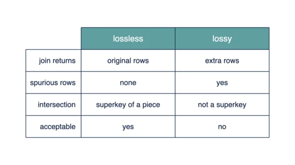
Lossless vs Lossy Decomposition: Comparison Table
| Aspect | Lossless Decomposition | Lossy Decomposition |
|---|---|---|
| Result of the natural join | Exactly the rows of R | Extra rows beyond R |
| Spurious tuples | None produced | One or more produced |
| Original relation recoverable | Yes, always | No, not exactly |
| Alternative name | Non-additive join decomposition | No standard alternative name |
| Condition on the intersection | Superkey of at least one piece | Superkey of neither piece |
| Acceptable in database design | Yes, the required standard | No, rejected outright |
| Effect on data integrity | Preserved exactly | Compromised by false rows |
| Relationship to functional dependencies | Confirmed by the FD tested | FD fails to hold across the pieces |
| What causes it | A split along a determinant attribute | A split along a non-determinant attribute |
| How it is detected | Apply the three-condition test | Same test fails on condition three |
| Relationship to normal forms | Guaranteed by BCNF decomposition | Not guaranteed by normal form alone |
| Effect on query results | Query results stay accurate | Joins return misleading extra rows |
| Typical exam framing | Verify this decomposition is lossless | Show this decomposition is lossy |
| Dependency preservation | A separate property, not guaranteed | A separate property, also not guaranteed |
Worked Example: The Same Table, Two Splits
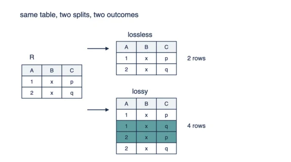
Here is one trace worth memorising for exams. Relation R holds three attributes, A, B and C, and exactly two rows.
| A | B | C |
|---|---|---|
| 1 | x | p |
| 2 | x | q |
The functional dependency A → B holds on R. That single FD decides whether a split survives the join test or fails it.
Split 1: R1(A, B) and R2(A, C).
The intersection of R1 and R2 is {A}. Since A → B, A determines all of R1, so A is a superkey of R1. Condition three holds.
R1 holds (1, x) and (2, x). R2 holds (1, p) and (2, q). Joining them on A returns exactly this:
| A | B | C |
|---|---|---|
| 1 | x | p |
| 2 | x | q |
So two rows come back, identical to R. This decomposition is lossless.
Split 2: R1(A, B) and R2(B, C).
The intersection here is {B}. B determines neither A nor C, so B is a superkey of neither piece. Condition three fails.
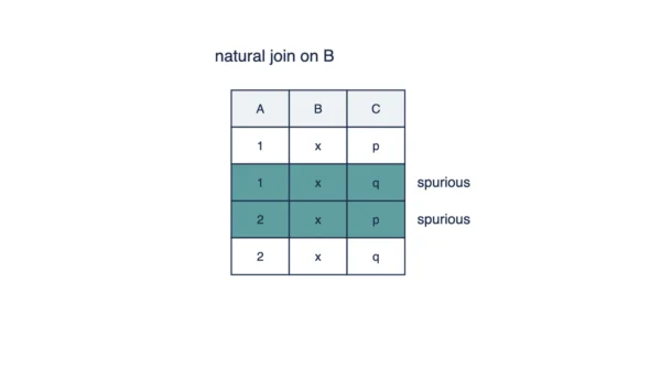
R1 holds (1, x) and (2, x). R2 holds (x, p) and (x, q). Joining them on B returns four rows, not two:
| A | B | C | Status |
|---|---|---|---|
| 1 | x | p | original |
| 1 | x | q | spurious |
| 2 | x | p | spurious |
| 2 | x | q | original |
Instead, four rows come back for two original rows. Rows (1, x, q) and (2, x, p) never existed in R; those are the spurious tuples. This decomposition is lossy.
Same table, same data, two different splits. Only the attribute chosen for the split decided whether the information survived. Notice, too, that the lossy join returned more rows than R, not fewer. So that is exactly why the name “lossy” confuses so many students.
How to Test a Decomposition
Testing a decomposition is mechanical once you know the three conditions. Apply them in order, and stop as soon as one fails.
- List the attributes of R1 and R2, and confirm their union equals every attribute of R.
- Find R1 ∩ R2. If it is empty, the decomposition is lossy immediately, no further check needed.
- Check whether R1 ∩ R2 functionally determines R1. If it does, the decomposition is lossless.
- If not, check whether R1 ∩ R2 functionally determines R2 instead. Either implication is enough.
- If neither implication holds, the decomposition is lossy, and the join will produce spurious tuples.
Applied to Split 1 above, the intersection {A} determines R1, so step three succeeds and the test stops there. Applied to Split 2, the intersection {B} determines neither piece. So step five is where the test lands, confirming a lossy result.
This test applies only to a binary decomposition. A schema broken into three or more pieces needs a different, iterative check, not this shortcut.
Where Students Lose Marks
- Thinking “lossy” means rows disappear. The join gains rows instead; nothing about it drops a row from R.
- Checking only condition one. The attributes adding up correctly says nothing about whether the join is safe.
- Requiring a superkey of both pieces. Condition three needs only one of the two, not both together.
- Forgetting the non-empty check. If R1 ∩ R2 is empty, the decomposition is lossy, whatever else holds.
- Assuming a higher normal form guarantees losslessness. Reaching Boyce-Codd Normal Form (BCNF) or Third Normal Form (3NF) does not excuse a decomposition from being tested directly.
Why Lossless Is Non-Negotiable
A lossy decomposition breaks every query that joins the pieces back together. So reports show rows that never existed. Totals inflate, and lookups return matches that are not real.
That risk, then, is why lossless-join decomposition stays mandatory, not optional, in relational design. A schema that reaches a higher normal form but fails the join test is not acceptable. Instead, it has to be redesigned, not shipped. So the same risk touches the strategy behind clustered vs non-clustered indexes. Both assume the joined rows are genuine.
Lossless-join and dependency preservation are two separate properties, and a decomposition can have one without the other. BCNF decomposition is always lossless, but it may not preserve every functional dependency. Instead, Third Normal Form decomposition can always achieve both together, one reason it stays the more common classroom target.
Interview Questions
Frequently Asked Questions
Wrapping Up
Lossless vs lossy decomposition comes down to one join, not a feeling. Test the three conditions on any split before trusting it. The union must cover every attribute. So the intersection must be non-empty, and it must be a superkey of at least one piece.
Keep the worked trace close for exams. For example, splitting R(A, B, C) on A stayed lossless. Splitting the same table on B produced two spurious tuples instead, (1, x, q) and (2, x, p). Same data, same table, and only the split decided the outcome.
Finally, remember that lossless-join and dependency preservation are separate checks. BCNF decomposition guarantees the first, not always the second. 3NF, by design, can guarantee both.
Related reading on DiffStudy:
- Logical vs Physical Data Independence
- Primary Key vs Foreign Key
- Clustered vs Non-Clustered Index
- File Systems vs Databases
- CS Fundamentals hub