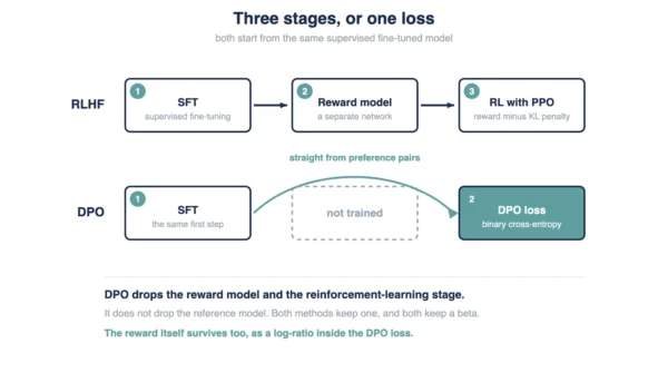
RLHF and DPO both start from the same preference pairs, one answer marked over another. RLHF trains a separate reward model first, then runs reinforcement learning against it, usually PPO. So DPO skips that separate network and the RL loop entirely. Instead, it optimises one binary cross-entropy loss straight on the preference pairs. Even so, a reward concept survives inside that loss. The paper defines an implicit reward there: β times the log ratio of policy over reference model. So DPO removes the standalone reward network, not the idea of reward itself. Both methods still depend on a reference policy, the same SFT model each one starts from.
Every alignment method starts from preference pairs, one answer marked over another. RLHF and DPO turn that ranking into a training signal in different ways, though. So RLHF adds a separate reward model and a reinforcement-learning loop. DPO instead folds preference learning into one loss on the base policy itself.
This guide leans on one source throughout: Rafailov and colleagues’ paper, “Direct Preference Optimization: Your Language Model is Secretly a Reward Model.” New readers should read our RAG vs fine-tuning guide before this one. That guide covers how a pretrained model becomes task-specific.
Why Alignment Starts With Preference Pairs
Both methods start from the same material. A prompt x goes to the SFT model, which produces two answers, y1 and y2. Then a human labeller marks one preferred, giving y_w ≻ y_l given x. So that single judgment call feeds everything downstream.
The paper models this ranking with the Bradley-Terry preference model. It assumes a latent reward function r*(x, y) behind every judgment. So the probability that y1 beats y2 follows one equation.
p*(y1 ≻ y2 | x) = exp(r*(x, y1)) / [ exp(r*(x, y1)) + exp(r*(x, y2)) ]
Since that ratio grows whenever r*(x, y1) outweighs r*(x, y2), a higher latent reward means a higher win probability. Neither RLHF nor DPO ever observes r* directly, though. Instead, both only see the pairwise labels, y_w over y_l.
How RLHF Works
The paper reviews RLHF as three phases. Each phase feeds the next, so skipping one breaks the chain.
- Supervised fine-tuning. A pretrained model is fine-tuned on high-quality task data, producing π_SFT.
- Preference sampling and reward learning. The SFT model generates answer pairs for each prompt, then human labellers rank them.
- RL optimisation. The policy is fine-tuned against the learned reward, commonly with PPO, sometimes REINFORCE.
Phase one updates the model’s full set of weights, the same cost our LoRA vs QLoRA vs full fine-tuning guide compares against lighter alternatives. Phase two samples each answer pair with the decoding controls covered in our temperature vs top-p guide.
Then phase three optimises this objective.
max over π_θ: E_(x~D, y~π_θ) [ r_φ(x, y) − β · D_KL( π_θ(y|x) ‖ π_ref(y|x) ) ]
β controls how far the policy may drift from π_ref, the reference policy. π_ref is the SFT model itself. The policy π_θ also starts from π_SFT, before RL optimisation pulls it toward higher reward.
How DPO Works
DPO collapses phases two and three into one step. Instead of training a reward model and then running RL, it optimises a single loss directly on the preference pairs.
L_DPO(π_θ; π_ref) = −E_(x, y_w, y_l)~D [ log σ( β log( π_θ(y_w|x) / π_ref(y_w|x) ) − β log( π_θ(y_l|x) / π_ref(y_l|x) ) ) ]
The paper describes this as “a simple binary cross entropy objective.” Its own Figure 1 caption states the goal plainly: DPO optimises for human preferences “while avoiding reinforcement learning.”
Three things disappear with that change. DPO needs no sampling from the language model during fine-tuning. Also, it needs no separate reward network. The paper adds that it avoids “significant hyperparameter tuning.” β still remains, though.
The gradient still has structure worth noting. It carries a dynamic, per-example importance weight, one that grows when the implicit reward orders a pair wrongly. Without that weighting, the paper reports, a naive version of the objective causes model degeneration. So in practice, the gradient increases the likelihood of y_w and decreases the likelihood of y_l.
RLHF vs DPO: Comparison Table
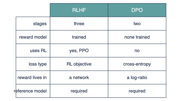
The table below lines up RLHF against DPO, field by field. Every value traces back to the paper’s own description of both pipelines.
| Aspect | RLHF | DPO |
|---|---|---|
| Training stages | Three: SFT, reward model, RL | Two: SFT, DPO preference loss |
| Separate reward model trained | Yes, r_φ(x, y) | No separate network |
| Reinforcement learning used | Yes, dedicated RL phase | No, avoids RL entirely |
| Optimiser or algorithm | PPO, sometimes REINFORCE | Gradient descent on the DPO loss |
| Loss type | Reward-model loss, then RL objective | Single binary cross-entropy loss |
| Where the reward lives | Inside a separate scalar network | Implicit, inside the policy/reference ratio |
| Reference model needed | Yes, inside the KL penalty | Yes, inside the loss itself |
| Role of β | Weighs the explicit KL penalty | Scales the implicit reward |
| Samples during training | Yes, y ~ π_θ during the RL phase | No LM sampling during fine-tuning |
| Offline vs online data | Online sampling in the RL phase | Offline, fixed preference dataset |
| Implementation complexity | Higher: reward network plus RL loop | Lower: one cross-entropy objective |
| Hyperparameter tuning | RL phase adds its own tuning | Avoids significant tuning; β still matters |
| What SFT provides | π_SFT seeds the policy and π_ref | π_SFT seeds the policy and π_ref |
| Preference model assumed | Bradley-Terry model, Eq. 1 | Bradley-Terry model, Eq. 1 |
| Gradient weighting | Standard PPO policy-gradient estimate | Dynamic, per-example importance weight |
| Needed at inference time | Nothing beyond the trained policy | Nothing beyond the trained policy |
One row deserves a second look, the reward’s location. RLHF keeps it in a separate network. DPO folds it inside the policy instead, as the next section explains.
The Reward Model DPO Removes
Phase two of RLHF trains a reward network, r_φ(x, y). So its loss follows directly from the Bradley-Terry model above.
L_R(r_φ, D) = −E_(x, y_w, y_l)~D [ log σ( r_φ(x, y_w) − r_φ(x, y_l) ) ]
This loss asks for one thing: score the preferred answer higher than the rejected one. Since σ squashes the difference into a probability, the network learns from ordering, not raw magnitude.
The paper notes this network is often initialised from the SFT model itself. A linear layer sits on top of the final transformer layer, the same stack covered in our self-attention vs cross-attention guide, producing one scalar reward. So the reward model is not a different architecture. It reuses the base model discussed in our BERT vs GPT guide, with a small head swapped in.
So DPO removes exactly this network, the standalone r_φ. What replaces it is the subject of the next section.
The Reward That Never Goes Away
DPO does not delete the reward. It reparameterises it instead.
The paper defines the reward implicitly represented by the policy and reference model this way.
r̂_θ(x, y) = β log( π_θ(y|x) / π_ref(y|x) )
So the reward becomes a log-ratio between the trained policy and the reference model. That change of variables, in the paper’s own words, “avoids fitting an explicit, standalone reward model.” The reward concept survives. So only the separate network disappears.
Explicit reward (RLHF):  r_φ(x, y)
Implicit reward (DPO):   β log( π_θ(y|x) / π_ref(y|x) )
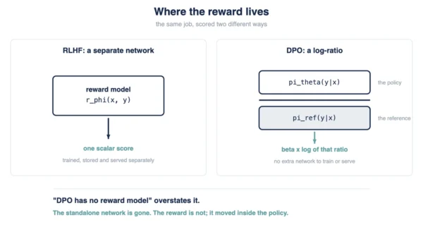
Both rows score the same thing, an answer y for a prompt x. RLHF scores it with a separate network. DPO scores it instead from two numbers already on hand, the policy’s probability and the reference model’s probability.
This is why “DPO has no reward model” overstates the case. The explicit, standalone network is gone, true. An implicit reward still sits inside the loss, defined by that same log-ratio.
The Two Losses Side by Side
Both training losses share one shape. Each one asks a policy or a reward network to prefer y_w over y_l.
Reward-model loss (RLHF): L_R(r_φ, D) = −E_(x, y_w, y_l)~D [ log σ( r_φ(x, y_w) − r_φ(x, y_l) ) ]
DPO loss: L_DPO(π_θ; π_ref) = −E_(x, y_w, y_l)~D [ log σ( β log( π_θ(y_w|x) / π_ref(y_w|x) ) − β log( π_θ(y_l|x) / π_ref(y_l|x) ) ) ]
Look at the term inside σ in each line. RLHF subtracts two scalar rewards from a separate network. DPO subtracts two implicit rewards instead, each a scaled log-ratio. Swap r_φ(x, y) for β log( π_θ(y|x) / π_ref(y|x) ), and the two losses collapse into the same form.
That is not a coincidence. It is the paper’s central claim: a language model is secretly a reward model, once its output is compared against a reference.
What Each Approach Costs
RLHF pays for its extra phase. It needs a reward network trained first, then an RL loop on top of that. Since the RL phase samples y ~ π_θ during training, it also needs infrastructure for that sampling.
DPO removes those costs, though not every cost. It still needs a reference model, π_ref, held fixed during training. β still needs a value, and the paper is explicit that DPO avoids significant hyperparameter tuning, not all of it.
Likewise, stability follows a similar pattern. RLHF’s RL phase inherits the tuning and sampling concerns of reinforcement learning generally. DPO instead trains on a fixed dataset with a single cross-entropy objective, closer to standard supervised learning.
One more cost applies to both equally. So neither approach adds anything at inference time. The deployed model is just the trained policy, whichever loss produced it.
When to Use Which
The choice tracks the trade-offs above, not a universal winner. The paper makes no such claim, and neither should a reader.
A team already running a stable RL pipeline can keep the reward model and PPO. That path adds a training stage, but it keeps the reward as an explicit, inspectable network.
A team that wants to skip the RL loop can adopt DPO’s single loss instead. That path removes the separate network and the sampling step, while keeping the same reference-model requirement.
Either way, the underlying assumption stays the same. So both methods trust the Bradley-Terry model to translate pairwise labels into a usable signal.
Interview Questions
Frequently Asked Questions
Wrapping Up
RLHF and DPO start from the same preference pairs and the same Bradley-Terry assumption. RLHF then trains a separate reward model and runs reinforcement learning against it. DPO instead folds both steps into one binary cross-entropy loss.
Remember the trap this page exists for. DPO does not delete the reward, it reparameterises it. An implicit reward, β log( π_θ(y|x) / π_ref(y|x) ), lives inside the DPO loss even though the standalone network is gone. So a reference model, π_ref, remains required by both methods too.
Related reading on DiffStudy:
- RAG vs Fine-Tuning
- LoRA vs QLoRA vs Full Fine-Tuning
- BERT vs GPT
- Self-Attention vs Cross-Attention
- Temperature vs Top-p